An overview of Alloy

In this first chapter we will explain how Alloy can be used to explore the design of a very simple software component, namely the well-known Trash or recycle bin present in most operating systems. The aim is to give a brief, at times superficial, overview of how to specify and analyse a software design with Alloy. The full details of the Alloy specification language and analysis techniques will be given in the following chapters.

The goal of the Trash is to enable deleted files to still be restored until an (undoable) action of emptying the Trash is made: when a file is deleted it is stored in the Trash; while still in the Trash, a file can be be restored; after emptying, all files contained in the Trash are permanently deleted.

More specifically, in this chapter we will show how Alloy can be used in the following tasks:

1. Formally specify, at a very abstract level, the design of the structure and behaviour of the Trash component.

2. Validate this design by simulation, namely using the Alloy Analyzer to check that it allows some of the expected behaviours of the Trash.

3. Elicit and verify some of the expected properties of the Trash component.

Specifying a software design

Transition systems are one of the most standard formalisms to reason about the behaviour of a system, and are a very convenient and abstract formalism to describe and reason about the design of a software system. A transition system contains the different states the system may be in while evolving over time, identifying which of these are possible initial states, and clearly depicting how the system can evolve by identifying the transitions that connect each state to every possible succeeding state.

The first step when specifying a transition system is to describe the structure of its states. In Alloy the structure of a system is described in terms of sets and relations. In Alloy parlance sets are called signatures, and are declared using the keyword sig followed by a mandatory signature name and an optional list of field declarations enclosed between braces. Fields are relations that connect elements of the enclosing signature to other elements. We will not use fields in this chapter, so our signature declarations in this example will always have a pair of empty braces after the name.

In Alloy, signatures are inhabited by the so-called atoms, elements without any internal structure or any particular semantics attached, and whose names will be automatically generated by the Analyzer. By default, in Alloy the value of all signatures and relations is immutable. To declare a mutable (or variable) signature just add the var keyword before the signature declaration.

Note

Alloy and Electrum.

The main difference of Alloy 6, when compared to previous versions of Alloy, is precisely the possibility of declaring mutable sets and relations. The reader may wonder if the previous versions of Alloy, where all signatures and relations are immutable, were in any way useful. In fact, in many software systems the main design problem concerns just structural aspects, for example, eliciting requirements about the data structures. We will give an example of this in the Structural design with Alloy chapter. Moreover, it was still possible to reason about behaviour with Alloy 5, by explicitly specifying the notion of time and of execution traces. However, this was often a rather time-consuming and error-prone task. The Electrum extension [FSE16] [ASE18] was proposed precisely to address this shortcoming. Electrum added an implicit notion of time, allowed the declaration of mutable signatures and relations, and the specification of properties with temporal logic. With Alloy 6, these extensions became a standard part of Alloy. For an overview of Alloy 5 check Alloy: A Language and Tool for Exploring Software Designs [CACM19] by Daniel Jackson or his excellent book Software Abstractions: Logic, Language, and Analysis [MIT12].

At a very abstract level, we can describe the state of the Trash component using two sets: the set of files existing in the file system at any time, and the subset of those that are currently in the trash. In our Alloy specification we will thus declare two mutable signatures: File and Trash, respectively. To signal that the latter is a subset of the former, in the declaration of Trash we will use the keyword in followed the name of the including signature. The Alloy specification of the Trash state is thus as follows.

var sig File {}
var sig Trash in File {}

In this example, the signature File is a top-level signature, one not contained in any other signature, while Trash is a subset signature. In Alloy all top-level signatures are disjoint. The same is true for mutable top-level signatures: they are always disjoint, even at different points in time, meaning that an atom cannot move from one top-level signature to another one in a state transition.

Having described the state of our system we can now proceed to specify its intended behaviour, namely what are the initial states and transitions of the Trash transition system. Unlike many formal specification languages, Alloy has no special syntax to declare this transition system. Instead it follows the idea, introduced by Leslie Lamport in the Temporal Logic of Actions [TOPLAS94], of specifying the transition systems implicitly by means of a temporal logic formula that recognises which are its valid execution traces. A trace is an infinite sequence of states, fully describing a possible behaviour of the system.

The formula specifying the transition system typically consists of two parts: one formula that specifies what are the valid initial states, and another that specifies which transitions are possible at each state. In the case of our example, in the initial state we have an empty trash bin. To test a set for emptiness we can use the keyword no followed by the set expression to be checked (to check that it is non-empty we can use the keyword some, and to check that it contains at most one element the keyword lone). To impose a constraint to restrict the valid traces of a system we can use the keyword fact followed by an optional name and a formula enclosed between braces. If that formula contains no temporal operators, namely if it is a normal first-order formula that constraints the values of the sets and relations in the state, then it is only required to hold in the initial state of every trace. In our example, the valid initial states can thus be specified by the following fact.

fact init {
  no Trash
}

To specify the valid transitions, it is easier to first think about the events (or operations) in the system. Each event will give origin to many transitions. In the case of the Trash component we have three events: delete a file, restore a file, and empty the trash. To specify an event, we will write a formula that holds in a particular state of a trace iff that event can occur in that state and the next state of the trace is a valid outcome of the event. These two conditions are usually called the guard and the effect of the event, respectively. To specify the effect we need to somehow evaluate the value of a formula in the next state or refer to the value of sets and relations in the next state. To evaluate a formula in the next state we precede it with the temporal operator after. To evaluate an expression in the next state we append it the operator '. For readability reasons, it is convenient to specify each event in a separate predicate. A predicate is a named formula that will only hold when invoked (for example in a fact). To declare a predicate the keyword pred should be used, followed by the predicate name, an optional list of predicate parameters, and a formula enclosed between braces. For example, the ‘empty trash’ event can be specified by the conjunction of three formulas as follows.

pred empty {
  some Trash and       // guard
  after no Trash and   // effect on Trash
  File' = File - Trash // effect on File
}

The first condition is the guard of our event, and it states that the trash can only be emptied in a state if the set Trash contains some files. After the guard we have two conditions to specify its effect. When specifying an event we should consider what is its effect on all mutable sets and relations that comprise the state. If nothing is specified about a particular mutable set or relation, then there will be no constraints restricting how that set or relation can evolve, meaning that it can change freely when the event occurs. If the intention was for that set or relation to remain unchanged when the event occurs, then an explicit formula stating that the value in the next state is the same as the present value must be added. Such “no change” effect conditions are usually called frame conditions. In the case of the ‘empty trash’ event, the first effect condition states that in the next state the Trash set will be empty (which could alternatively be specified by no Trash'), and the second effect condition states that the value of the File set in the next state is the result of subtracting the set of files in the Trash from its current value (operator - denotes set difference, & set intersection, and + set union).

Tip

Increasing the readability of your specification.

Alloy has a dual syntax for Boolean operators: they can be both written with the typical programming language style operators, but also using the respective English words. We have ! and not for negation, && and and for conjunction, || and or for disjunction, => and implies for implication, <=> and iff for equivalence. Alloy syntax was designed to be very clean and readable. The use of the English version of the operators further increases the readability of the specifications, and will be the preferred style in this book. Additionally, in a fact or predicate, formulas written in different lines are implicitly conjoined, so the and keywords at the end of the first two lines in the empty predicate are not needed, and omitting them further increases the readability of the event specification.

The ‘delete file’ event occurs when a file (not currently in the trash) is moved to the trash bin. This event can be specified by the following predicate, parametrised by the file to be deleted. Notice the frame condition on File: moving a file to the trash bin does not permanently delete it, and so the set of files in the file system remains unchanged.

pred delete [f : File] {
  not (f in Trash)   // guard
  Trash' = Trash + f // effect on Trash
  File' = File       // frame condition on File
}

Important

Everything is a set!

The attentive reader might wonder how the expression Trash + f in this predicate type checks, since the union operator is being applied to the set Trash and the file atom f. In Alloy every expression denotes a set, and in particular the value of a variable is a singleton set containing just the value of that variable. So the f in Trash + f is a set of files, just like Trash, and it is possible to compute the union of both. This may seem rather strange at first, but it is one of the nice details of Alloy, that further contributes to simplify its semantics and syntax (by substantially reducing the number of operators in the language). Another example is the in operator which in fact tests for set inclusion and not set membership, as one might expect. Again, since f denotes a singleton set, expression f in Trash is indirectly checking whether f is a member of Trash, so the same in operator can easily be used for both purposes.

The ‘restore file’ event specification is very similar to the one of the ‘delete file’ event.

pred restore [f : File] {
  f in Trash         // guard
  Trash' = Trash - f // effect on Trash
  File' = File       // frame condition on File
}

Having specified our three events, we now need to constrain the valid transitions of the system. This can be done by imposing through a fact that, at each possible state during the system evolution, one of the three events must hold. To impose a constraint on all the states of a trace, we can use the temporal operator always followed by the desired formula. With this operator we can easily specify the valid transitions of our Trash component example as follows.

fact trans {
  always (empty or (some f : File | delete[f] or restore[f]))
}

Note the usage of the existential quantifier some to “pick” at each state a file to be deleted or restored.

Validating a design specification

Now that we have a first specification of the intend behaviour of the Trash component, and before proceeding with the verification of its expected properties, it is advisable to validate it to get some assurance that indeed it behaves as expected. A typical way to perform such validation is by using some sort of user-guided simulation. The Alloy Analyzer has several mechanisms to allow the user to explore and validate a design, including an interactive exploration mode akin so simulation [FIDE19].

A distinguishing feature of Alloy is that analysis commands can be included together with the declarations and facts in a specification. There are two analysis commands, both accepting either a predicate or a formula enclosed in braces (and in this case an optional command name): run commands instruct the Analyzer to check the satisfiability of the formula (and the declared facts), yielding a satisfying instance if that is the case; check commands instruct the Analyzer to check the validity of the formula (assuming the declared facts to be true), yielding a counter-example instance if that is not the case. In the case of specifications with mutable sets and relations, an instance is a valid execution trace, an infinite sequence of states, each a valuation of the declared sets and fields.

Note

Instances or models?!

When presenting the semantics of a logic, instances of formulas are usually known as models: a model of a formula is a valuation of its free variables that makes the formula true. In Alloy the term model is frequently used to denote the specification of a system, and the term instance is used to denote a satisfying valuation. This use of the term model in Alloy parlance is consistent with other techniques and languages for software design, namely the Unified Modeling Language, where a software model is precisely the kind of artefact we have been denoting by a specification.

Another distinguishing feature of Alloy is that the instances returned by the analysis commands are depicted graphically as graph-like structures: atoms belonging to the different sets are nodes (depicted as boxes by default) and relations are edges (depicted as arrows). Moreover, this graphical depiction can be customised using themes, namely it is possible to customise the colours and shapes of nodes and edges according to the sets and relations they belong to.

The usual way to start validating a specification is to define an empty run command: an empty formula is equivalent to true, and this command basically asks for an instance that satisfies all the declared facts. If none is returned then the facts are inconsistent and most likely our specification of the system is buggy and needs to be corrected. To kick-start the simulation process we will add an empty command (named example) to our specification.

run example {}

To execute the single command of a specification, or to re-execute the last command, just press cmd-e or the Execute button in the toolbar of the Analyzer window. If you have multiple commands, to choose which one to execute go to the Execute menu and select the desired command. If the commands are named you will see the names there, otherwise you will see an automatically generated name composed by the type of command (run or check) followed by a $ and a sequential numeric identifier. After executing the example command we get the following instance.

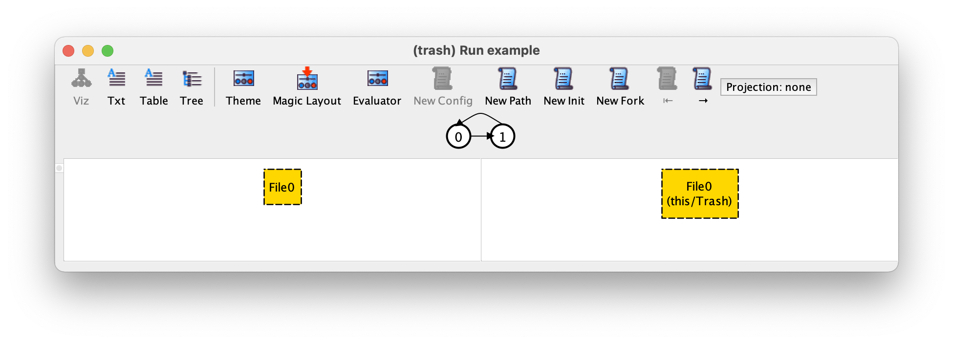
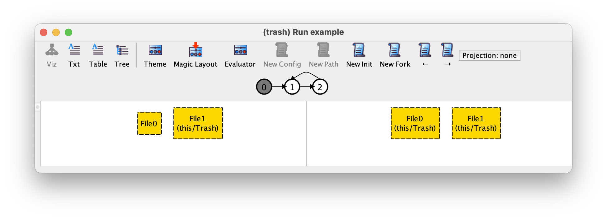
Here we see a depiction of an execution trace that satisfies our specification. Below the toolbar, the Alloy visualiser shows a depiction of the instance trace, which in this case consists of two states, with the second being followed by a loop back to the initial one. This trace is thus an infinite alternating sequence of the two states. All traces returned by the Alloy Analyzer will be of this kind: a finite sequence of states followed by a loop back to one of the previous states. All the execution traces are infinite but the tool only returns and depicts traces that can be represented finitely using a back loop. In the lower part of the window the visualizer focuses on a particular transition of the trace, depicting the pre- and post-state in the typical Alloy style: the atoms are named sequentially according to the signature they belong to, and atoms belonging to a subset signature (such as Trash) are labelled with that signature name. Mutable sets (and relations) are drawn with dashed borders by default, but this can be changed in the theme. The two states being depicted are the ones shown in white in the trace, all will be kept centred in the trace depiction. When the visualizer window pops up the transition being depicted is always the first one, with the state on the left-hand side being the initial state of the trace. In this example, we can infer that the first transition was due to a file deletion: initially we have a file that is not in the trash, and in the second state this file is in the trash: the only event that could have caused this transition is a deletion.

To navigate in the trace, namely to move forwards and backwards to focus on a different transition, just press the → or ← buttons in the toolbar (or cmd-→ and cmd-←), respectively. For example, by moving forward to focus on the second transition we get the following.

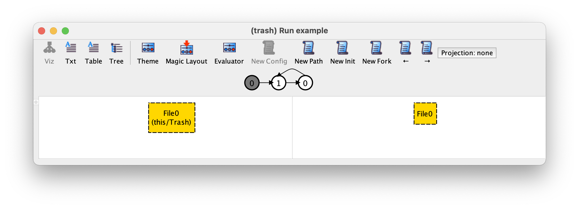
The second transition was caused by a ‘restore file’ event: in the pre-state File0 is in the trash and in the post-state it is no longer there. As such we can conclude that our first instance is an infinite alternation between deleting and immediately restoring File0, which is a valid execution of the system.

Note

Displaying the event corresponding to a transition.

The Alloy instance visualiser does not show the event that corresponds to a transition. Actually, there is no notion of event in Alloy: our events were modelled by three normal logic predicates, so there is no way for the visualiser to know these are events that should be treated specially. Another problem is that a transition may not correspond to just one event: oftentimes two different events can originate the same transition, and at this abstract level of specification there is no way (nor interest) in distinguishing which one actually occurred. In most examples, namely simple ones like our running example, it is kind of trivial to infer which event occurred. However, in some more complex designs that is not the case. In section An idiom to depict events we will present an Alloy idiom that allows the visualisation of the name (or names) of the events that could have caused each transition.

In the toolbar of the Alloy instance visualiser window we can find three buttons, that can be used to ask the Analyzer for alternative instances:

New Config

This button asks for a new trace that differs in the values of immutable sets and relations. Usually, immutable elements constitute the configuration of a system (for example, describing a specific network topology where a protocol is to be executed), and by pressing this button we will get an execution trace with a different configuration. In this example, all our sets are mutable, so this button is not applicable and is greyed out.

New Path

This button asks for a new (different) execution trace (a.k.a. path).

New Init

This button asks for a new trace with a different initial value for mutable sets and relations, allowing us to quickly explore a scenario starting with different initial conditions.

New Fork

Finally, this button asks for a different trace with the same behaviour up to the (left-hand) pre-state we are currently focused, but a different transition at this point. If that is possible, the pre-state will remain the same and we will see a different post-state. The latter could be a different result for the same (non-deterministic) event, or the outcome of a different event.

For example, if at this point we press New Init we could get the following instance.

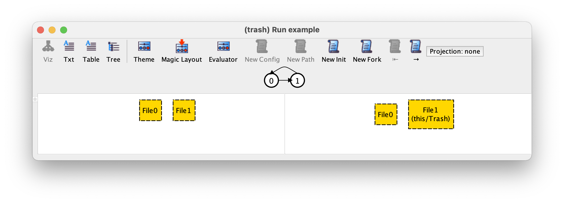
We now have two different files at the initial state, and only File1 is deleted. If we press → we can see that in the second transition this file is restored back.

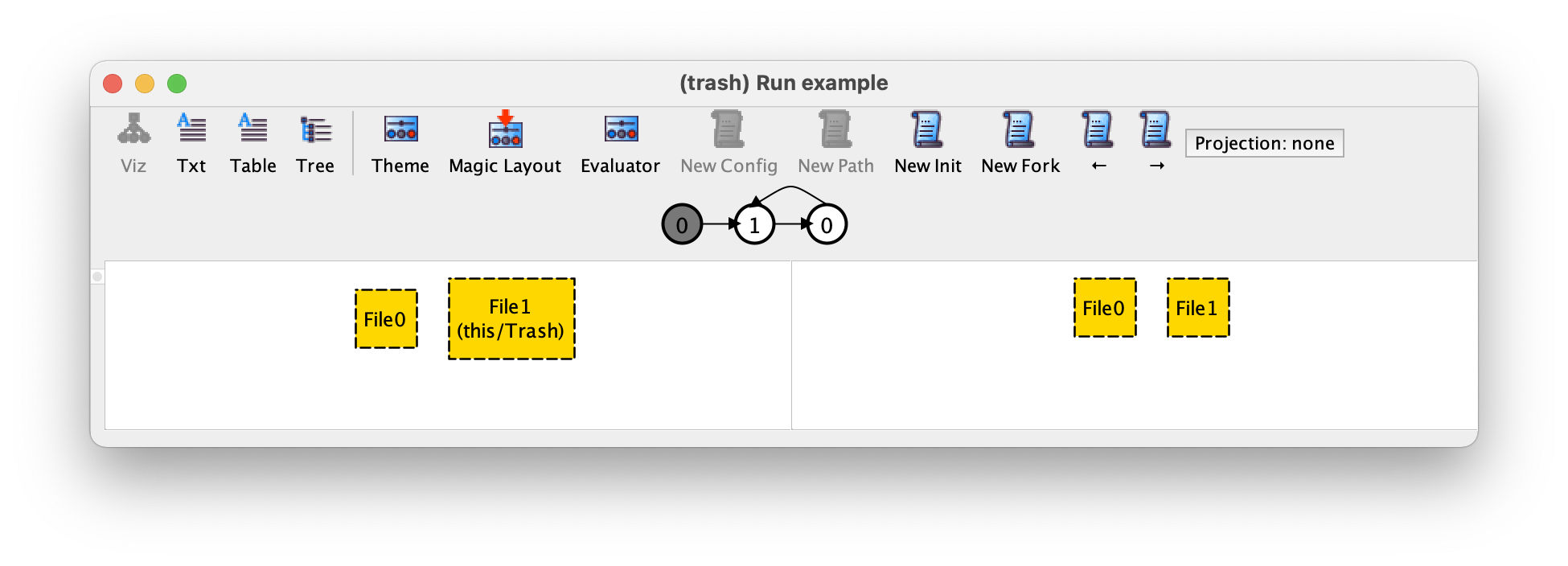
If now we press New Fork we get the following trace.

In this trace, the second transition is another deletion (of file File0) instead of a restore (of File1). Our trace now starts with a deletion of File1 followed by an infinite alternation of deleting and restoring File0. The New Fork is the main tool used while validating a design specification, since it allows us to explore alternative behaviours in a very similar way to simulation in other formal verification or model checking tools.

Before proceeding with the validation of our design, let’s customise our visualisation, for example by setting a different colour for files in the trash. To do so just press the Theme button in the toolbar. On the left-hand side you will see many theme customisation options. Just select the set Trash, and in the first drop-down menu on the top left-hand select the colour red, as follows.

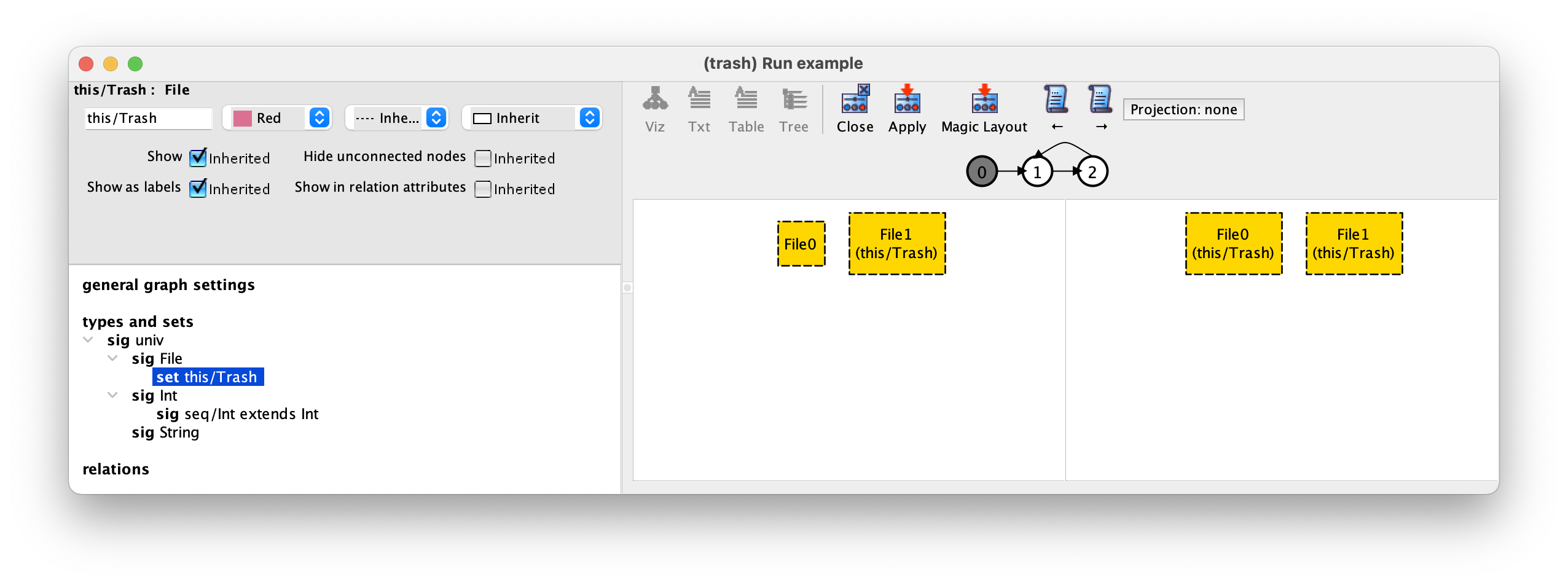
After selecting Apply in the toolbar and then Close our trace will now be displayed as follows.

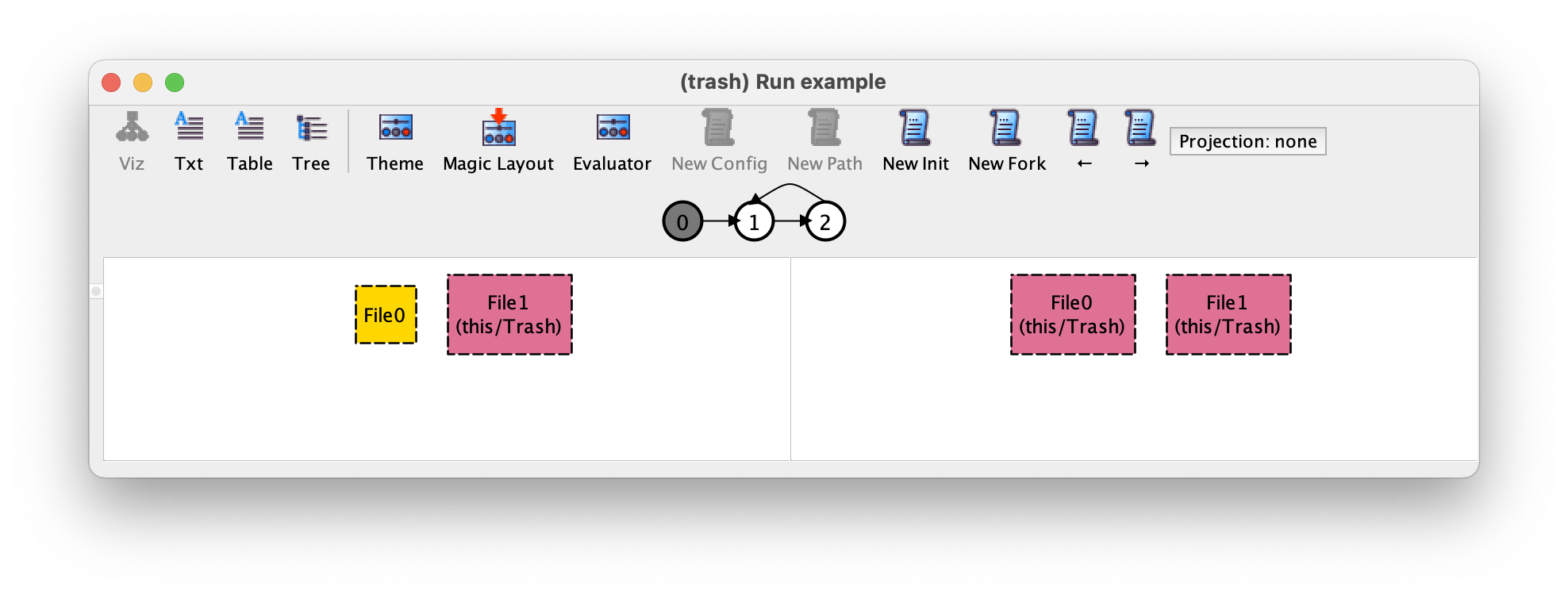
There are many options in the theme customisation menu, and when dealing with larger more complex systems this will become an extremely useful feature to help better understand execution traces. We will further discuss themes and give some tips about how to use them in the advanced-validation chapter.

If we now press New Init, to again ask for a different initial valuation of our sets, we get the following trace, where initially we have three files in the file system instead of two.

By pressing New Init one more time we get the following message.

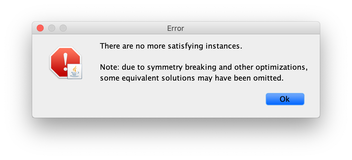
This may seem rather surprising at first. First, why isn’t the Analyzer returning instances where, for example, initially we have more than three files!? Second, why isn’t the Analyzer returning instances where, for example, initially there are two files named File1 and File2 instead of File0 and File1 as above!? The former situation is due to scopes. To enable automatic analysis, Alloy imposes a bound on the size of all signatures. This bound is defined by a scope on commands. By default the scope is 3 for all top-level signatures, meaning that instances will only be built using at most three atoms for each top-level signature. This scope can be changed by using the keyword for after a command, followed by the desired global scope for all top-level signatures. It is possible to set a different scope for specific signatures, by following this global scope by the keyword but and a list of comma separated scopes for different signatures. For example, if our run command was instead

run example {} for 5

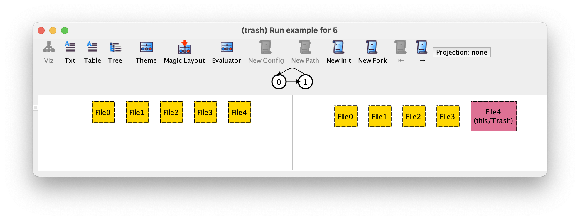
the scope of all top-level signatures, in this case only File, is set to 5. If we pressed New Init a few times we could get the following instance.

The second omission is due to symmetry breaking. As mentioned before, atoms have no semantics attached. In particular, the names the Analyzer creates for them are meaningless: File0 isn’t the name of a particular file existing in a real-world file system, but just a random name to help us distinguish it from other files. As such, two instances that only differ in the names of the atoms are in fact the same instance (they are isomorphic up to atom renaming), and showing both to the user would just encumber the understanding of the specification. To avoid this, and also to speed up analysis, the Analyzer implements a powerful symmetry breaking mechanism that excludes from the search most isomorphic (symmetric) instances.

To conclude our validation let’s try to find a concrete trace example using the Analyzer, namely one where initially we have a single file, which is then deleted, and finally the trash is emptied. To do so we re-execute our example run command, obtaining the desired initial state.

We then press → to move to the second transition, which corresponds to the recovery of the previously deleted file.

Then, to ask for a different transition, namely one corresponding to a trash emptying event, we press Fork. Surprisingly, instead of different next state with no files, we get the no more satisfying instances window!

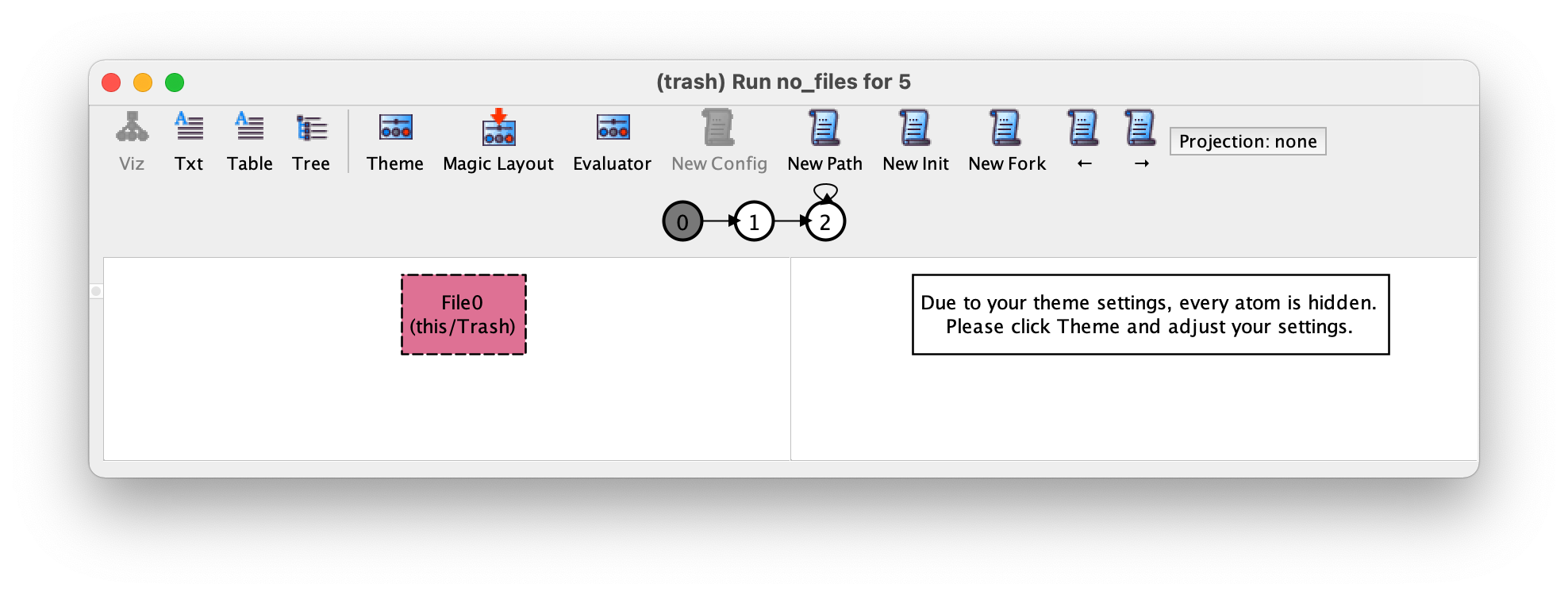
This means that this execution trace, which for sure we want to allow in our system, is not currently considered valid according to our specification. In fact, the current specification does not allow all files in the file system to be permanently deleted, as we can confirm by defining the following run command, now with a formula, which asks for a trace where we reach a point where eventually there are no files. Executing this command yields no instances, which clearly indicates that our specification is wrong.

run no_files { eventually no File } for 5

In this command’s formula we used the temporal operator eventually: a trace satisfies this operator if the ensuing formula is true at least on one of the states of the trace.

So what is the problem with our specification? The issue is that fact trans imposes that at any point in time one of the three events (delete, restore, or empty) must occur. Since empty has a guard requiring the trash to have some files, and the other two events also require the existence of at least one file, none of these three events can occur when there are no more files. This means that it is impossible to have an infinite trace where one of the states has no files, since no transition would be possible at that point. To fix our specification there are many options. We could, for example, specify an event allowing the creation of new files. Or, to keep the focus of our specification just on the Trash component, we could add an event that captures the (very real) possibility that the user of our system is doing something else in the system that does not affect the trash bin. When considering only the sets in our abstraction of the trash bin, this event will have no effect at all, so the specification of this event consists only of frame conditions.

pred do_something_else {
  File' = File
  Trash' = Trash
}

Having this predicate, we can now fix our specification of the valid transitions as follows.

fact trans {
  always (empty or (some f : File | delete[f] or restore[f]) or do_something_else)
}

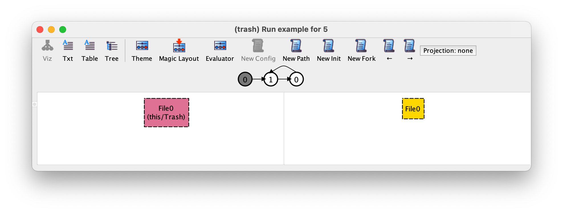
If we now re-execute the no_files command we get the following instance, where we basically never have any files, which, although a bit surprising, should be considered as a valid instance of our design.

Note

A quicker way to detect our problem.

The attentive reader could notice that actually the problem with our specification could have been detected earlier in this validation process. With the example command, when pressing Next Init to get instances with a different number of files in the initial state, after getting an instance with three files the no more satisfying instances popped up. At this point we could have noticed that the Analyzer was not yielding an instance with no files at all in the initial state, something that should have been possible.

To search for an instance where initially we have some files but eventually they are all permanently deleted we could either do a “simulation” starting with command example and using → and New Fork until we get to a point where the trash is empty, or just change the no_files command to search directly for such an instance.

run no_files {
  some File
  eventually no File
} for 5

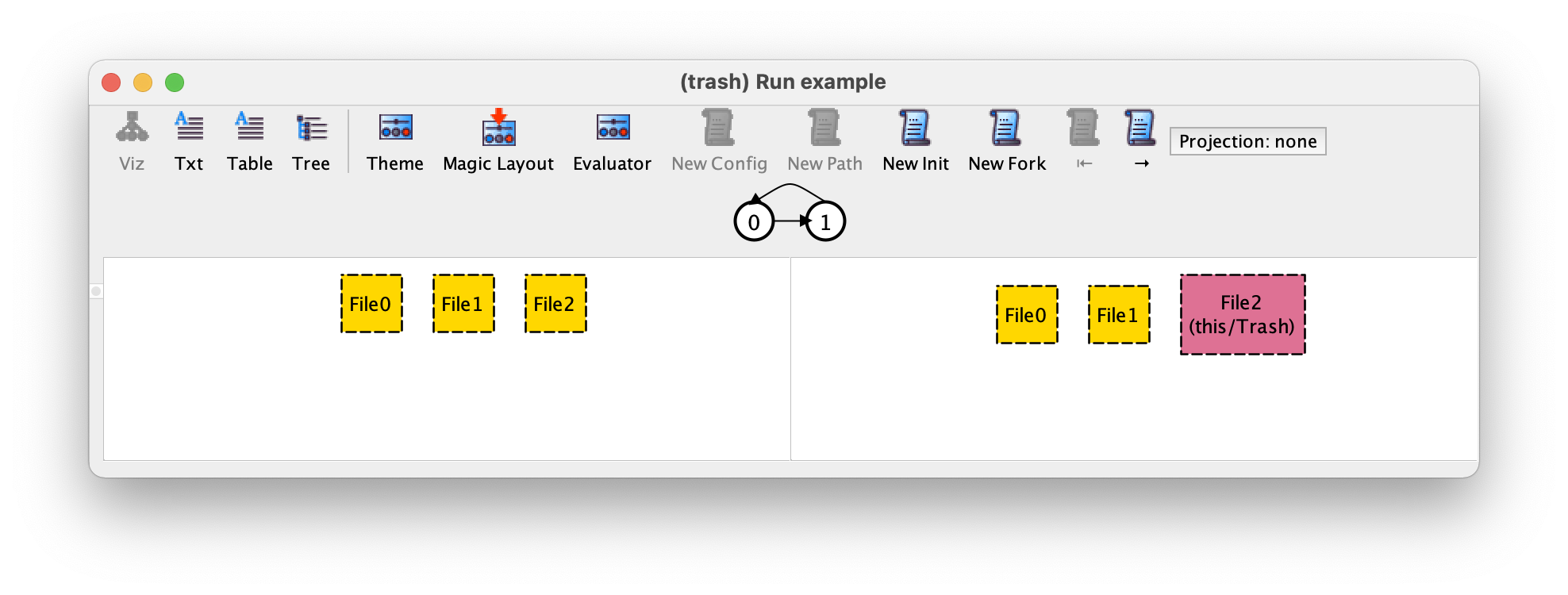
Recall that without any temporal operator, the added constrain applies only to the first state. Executing this command yields an instance with a single file that is immediately deleted. By pressing → we get to the following transition corresponding to the emptying of the trash.

Verifying expected properties

After validating our design we now proceed with the specification and verification of some of its expected properties. To exemplify, we will consider the following (rather trivial) properties, but many more could be specified about this example.

1. Every restored file must have been previously deleted.

2. If all files are in the trash and we empty it then no more files will ever exist.

A nice thing about Alloy is that the same logic is used to both specify the system and its expected properties. In many formal specification languages and verification tools (namely, most model checkers), a different language is used for each. In Alloy we use temporal logic, of which we already saw some of the key operators, namely always and eventually. So far our formulas consisted of exactly one of these operators followed by some constraint, so the meaning of the formula was easy to grasp: in the case of always, the ensuing formula must be true in all states of a trace for it to be considered a valid instance, and in the case of eventually the formula must be true at least in one state. However, formulas can contain several of these operators, potentially nested, which further complicates their understanding. As detailed in the A temporal logic primer chapter, a temporal formula is in fact evaluated in a particular state of a trace. The outermost formula is evaluated in the initial state, but nested temporal formulas may be evaluated in different states of the trace depending on the enclosing temporal operator. So, the (informal) semantics of the temporal operators is the following:

always

When evaluated in a particular state, the ensuing formula must be true in that state and all the following states.

eventually

When evaluated in a particular state, the ensuing formula must be true in that state or in at least one of the following states.

after

When evaluated in a particular state, the ensuing formula must be true in the next state (which always exists, since traces are infinite).

We will now introduce a couple more temporal operators that may come in handy. These temporal operators are of a different nature of the above, because they constrain the past behaviour, while those we have seen so far constrain the future behaviour.

historically

When evaluated in a particular state, the ensuing formula must be true in that state and all the previous states.

once

When evaluated in a particular state, the ensuing formula must be true in that state or in at least one of the previous states.

Properties to be verified by check commands should be written in assertions. An assertion is declared with the keyword assert, followed by an identifier, and a formula enclosed between braces. For example, the first property above could be specified as follows.

assert restore_after_delete {
  always (all f : File | restore[f] implies once delete[f])
}

Here we have an example of a nested temporal operator. The outermost always imposes that the formula all f : File | restore[f] implies once delete[f] is true in all states of the execution traces. The all in this formula is an universal quantifier, meaning that in all states restore[f] implies once delete[f] must be true for every file f in the file system at that state. This formula imposes that whenever the ‘restore file’ event for a particular file is observed in a state, the ‘delete file’ event for that very same file must have been observed before. To verify this assertion we can use a check command followed by the assertion name to be checked.

check restore_after_delete

This command yields no counter-example instances, meaning that the assertion is most likely valid. Note that the command has an implicit scope on top-level signatures, so this result means that the assertion is valid for file systems with up to 3 files. In Alloy, commands also have a scope on the size of the finite prefix of traces that precedes the mandatory back loop. By default this scope is 10, meaning that the verification only checks for counter-example traces with at most 10 different states (and transitions). This is a verification technique known as bounded model checking. The Alloy Analyzer searches for counter-examples of increasing length, and is guaranteed to return the shortest one, if some exists. To change this bound just set the scope of the special signature steps. For example, to verify the above property for file systems with up to 5 files and traces with at most 20 different states the scope could be set as follows.

check restore_after_delete for 5 but 20 steps

This command also yields no counter-examples. With such a large scope it is thus very likely that our property is indeed valid. Although the analysis is always bounded in respect to the signatures, we can perform unbounded model checking (or complete model checking) in respect to the size of the traces, essentially verifying properties for traces composed by an arbitrary number of states. To do so we must first choose a solver in the Options menu that supports unbounded model checking. At the moment only the nuXmv solver supports that feature. The solver is the analysis tool that the Analyzer uses in the backend to perform the actual search for instances and counter-examples. For bounded model checking, many different solvers can be used: some of them may be considerably faster than others in particular examples, so it is always worthwhile to try them out if your analysis commands are very slow. To verify our property for file systems with up to 3 files and traces of any length the scope could be set as follows.

check restore_after_delete for 3 but 1.. steps

Again, no counter-examples are found!

The second property can be specified as follows.

assert delete_all {
  always ((Trash = File and empty) implies always no File)
}

Basically, in every state where the formula Trash = File and empty holds (all files are in the trash bin and the ‘empty trash’ event occurs) the formula no File (no files exist) must forever hold. To verify this property (with bounded model checking) we could issue the following command.

check delete_all

Surprisingly, this command yields the following counter-example with three different states, of which we show the first two transitions.

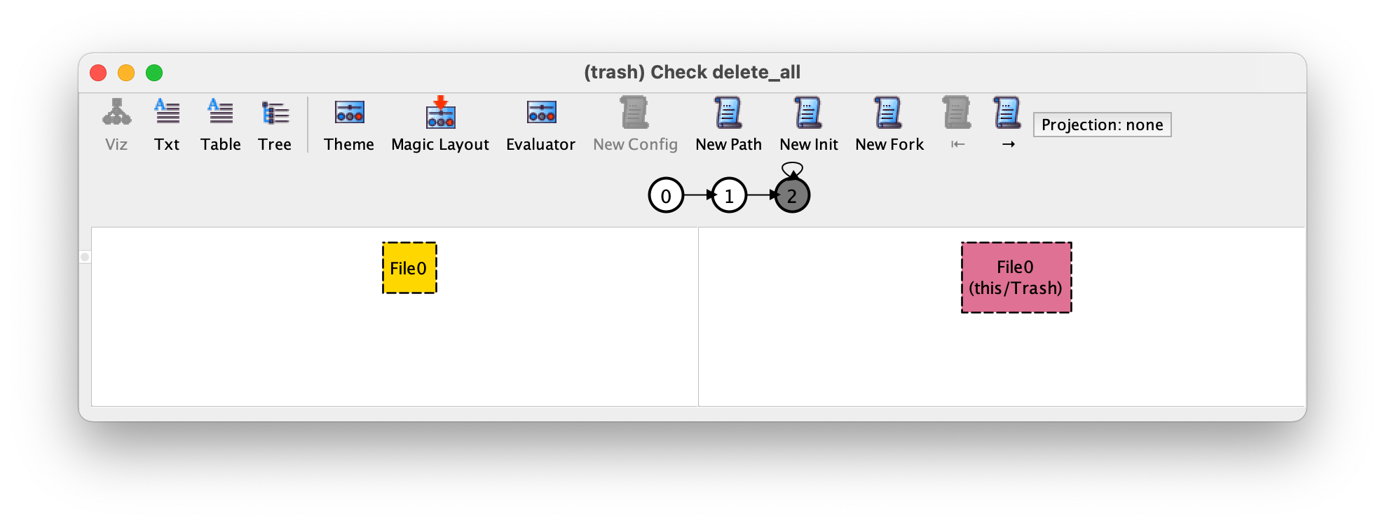
Notice that this is exactly the same instance we got when running the no_files command. On first sight, this trace does not look like a valid counter-example, since after deleting the only existing file and emptying the trash the file system remains forever empty. The problem in this case is that our specification of the property is buggy (and not the specification of the system, which hopefully is still correct). The semantics of the temporal operator always requires the ensuing formula to also hold at the state where the formula is evaluated, so in the above specification we were actually demanding that the file system is empty also in the same state where the ‘empty trash’ event occurred. This is not what we wanted: instead we should have required that the file system remains forever empty, but starting only in the (post-)state after the occurrence of the ‘empty trash’ event. We could fix our specification of the property by adding an after operator before the innermost always.

assert delete_all {
  always ((Trash = File and empty) implies after always no File)
}

Now the check command no longer yields a counter-example, and we can conclude that our Trash component design most likely satisfies these two properties!