Alloy modelling tips
As Alloy specifications increase in size in complexity, it becomes harder to comprehend them and interpret their instances. This chapter explores some modelling and validation tips that can be followed to ease this task, ranging from the usage of intelligible idioms to advanced features of the Analyzer’s instance visualizer.
Improved visualisation with derived relations
You might have realised that the instance visualizer plays an essential role in the validation of Alloy specifications. A key feature in this process is the ability to customise the theme so that the relevant information is highlighted (and the irrelevant one hidden). In this section we present another feature of the visualizer that allows further tweaking instance visualization: the introduction of derived relations.
Derived relations in Alloy are introduced through the declaration of
functions (much like derived formulas are introduced through the declaration
of predicates). These are declared with
the keyword fun, followed by the function name, an optional list of
function parameters, its return type, and an expression enclosed between
braces. The return type can be any relational expression with arbitrary arity.
Once declared, these functions can be freely used in relational expressions.
Let’s get back to the file system example from chapter Structural design with Alloy. A function could be declared to retrieve, for instance, all empty directories, which would be defined as follows.
fun empty_dirs : set Dir  {
  Dir - entries.Entry
}
At first sight, if we wanted to show the set of empty directories when
visualizing an instance, we would have to declare an additional subset
signature and enforce in a fact that its value is equal to the set
empty_dirs. However, this signature would have to be solved by the
Analyzer without actually introducing anything new in the specification.
Besides the obvious benefit of declaring re-usable expressions, Alloy
functions without parameters have an additional interesting feature: they
are introduced by the visualizer in the depiction of instances, and are shown
along the declared signatures and fields. Moreover, since they are introduced
by the visualizer after the solving process, they can be freely abused without
undermining the performance of the analysis. For instance, running the last
version of the example command from chapter Structural design with Alloy,
will now yield the depiction below.
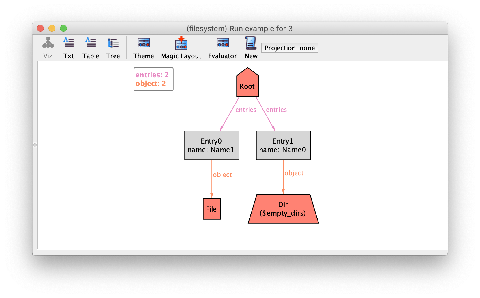
Notice how the empty directory at the bottom has an additional label
$empty_dirs. All visualization elements introduced by the visualizer
are prefixed with a $. Since empty_dirs returns a set, it is
interpreted as a subset of Dir which by default are shown as labels in
the theme. As expected, their depiction can be customised as any other
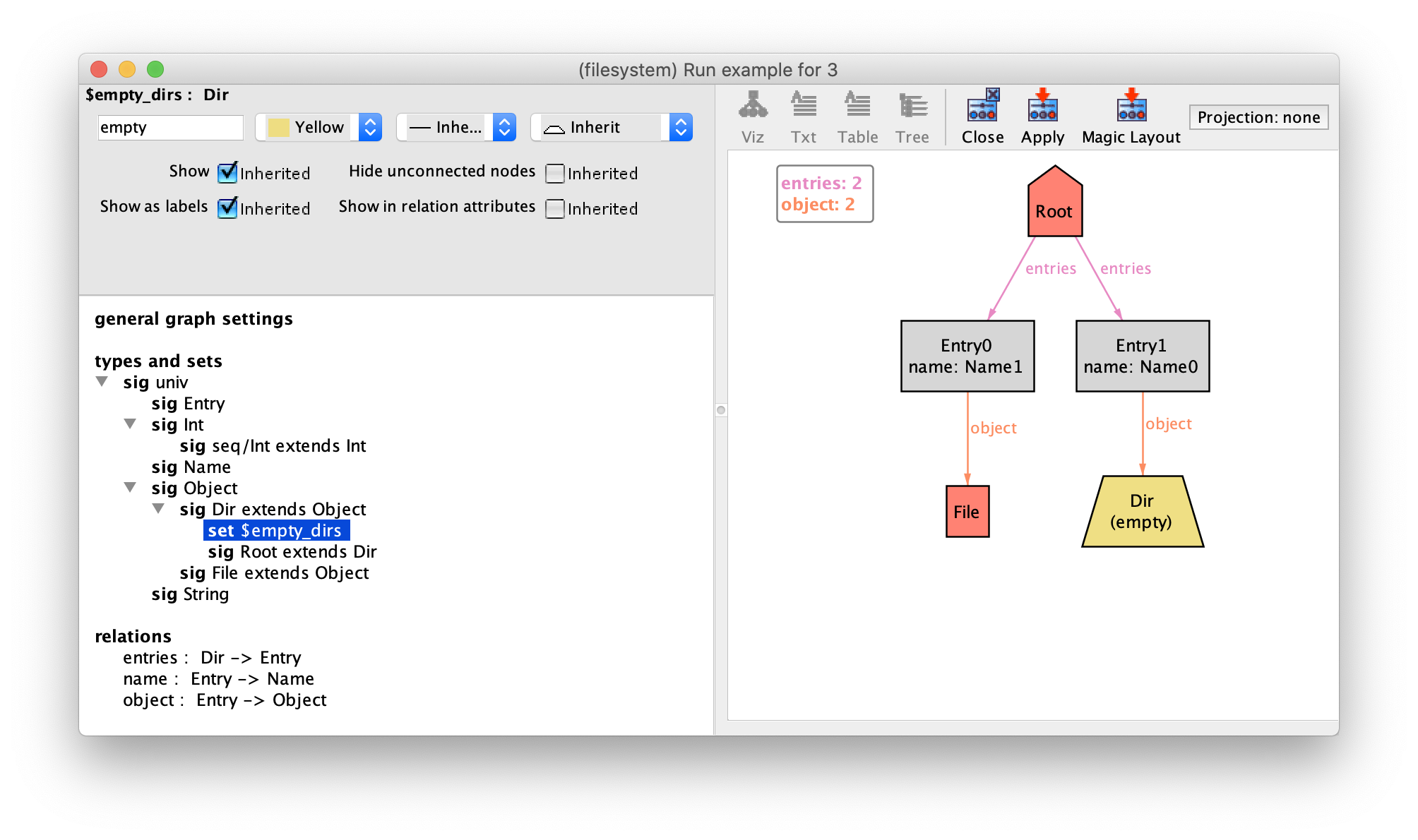
signature. For instance, to highlight empty directories in the depiction, open
the theme customisation menu, set $empty_dirs to be coloured in yellow
and the displayed name to empty. The resulting depiction is below,
where empty directories are clearly distinguished from non-empty ones. You
could also hide the label altogether and just change the colour of empty
directories by just setting to Show as labels to Off
for empty_dirs.
Note
What’s with these other $-prefixed variables?
You may have noticed that sometimes $-prefixed sets (or relations)
appear in the visualizer even without derived functions declared in the model. This is
because some existential quantifications in run commands (or universal ones
in check commands), are solved through a process known as Skolemization.
This process involves creating a relation corresponding to a witness of the
quantification to which the solver will attempt to assign a value. Besides
improving the performance of the analysis if used sensibly (the depth level
can be configured in , with 2 as
default), this actually allows the execution of commands with certain
higher-order quantifications.
Since these variables are solved by finding a value to a relation, they can
also be depicted when visualizing the instance. This is useful since it helps us identify
witnesses of quantifications. Their name is prefixed with $ and the
context in which the quantification occurs. Consider, for instance, the
following command.
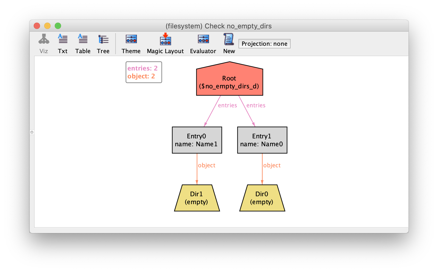
check no_empty_dirs {
  all d : Dir | d in empty_dirs }
The universal quantification on a check will be solved through
Skolemization. This property is obviously false, and returned
counter-examples have assigned a value to the Skolem relation of d
that has broken the property. Since the context of the quantification is the
no_empty_dirs command, the Skolem relation is named
$no_empty_dirs_d.
Like any other subset signature, the visualization of Skolem relations can be configured in the theme, and they can be hidden if we feel they are cluttering the depiction.
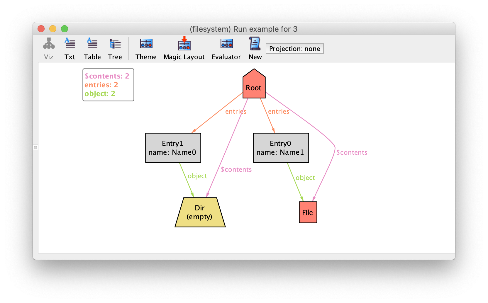
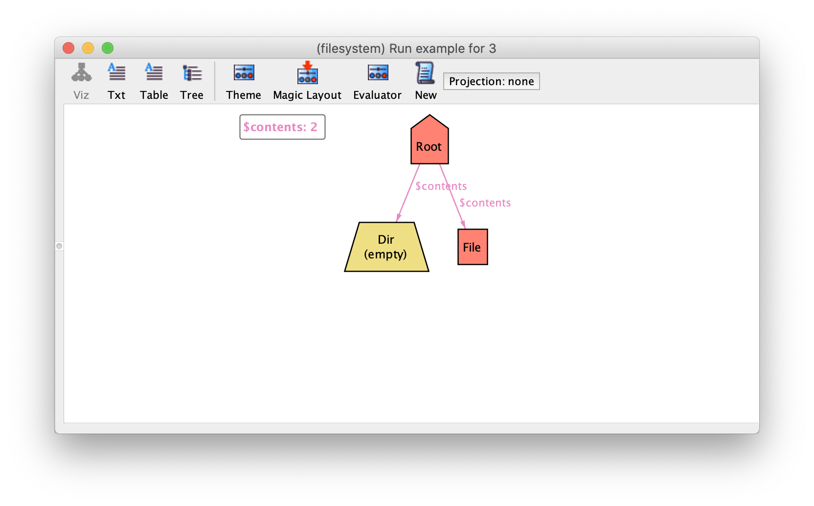
Derived functions without parameters are actually introduced by the visualizer regardless of its arity, resulting in additional edges for relations of arity higher than 1. For instance, if we wanted to depict directly the relation between directories and their content, hiding the entry atoms in the middle, we could define the binary relation below.
fun contents : Dir -> Object {
  entries.object
}
Running the command again results in the depiction below, with
$contents edges directly between directories and objects.
Once we start introducing derived relations, it is often useful to hide others
elements in order to unclutter the visualizer. In this case, we simply set
Show to Off for the Entry signature, resulting
in the depiction below where the content of directories is evident.
A consequence of short-circuiting entries in the visualizer is that we can no
longer see the name of the objects inside a directlry. Relations with arity
higher than 2 are depicted in the visualizer as edges with labels. Thus, a
ternary relation with type Dir->Name->Object could be used to keep the
content edges between directories and objects but also show the name of the
object. Defining such relations is often not trivial, and usually requires
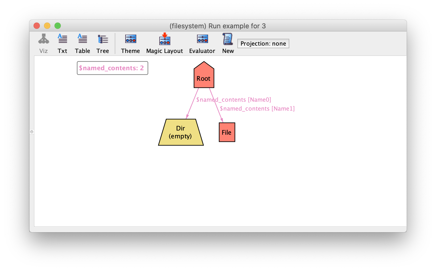
defining relations by comprehension. In this case this ternary relation could
be defined as follows.
fun named_contents : Dir -> Name -> Object {
  { d : Dir, n : Name, o : Object |
    some e : Entry | e in d.entries and e.name = n and e.object = o }
}
Here, we are collecting all triples d->n->o such that there is an
entry in d that has name n and object o. The resulting
depiction is shown below, where the labels of relation $named_contents
have the names of the objects appended.
Although we focused on an example without mutable signatures or fields, this strategy also works in that context, as we shall see in section An idiom to depict events. That’s because derived relations are evaluated in the state they are called from, and when depicting traces, the visualizer will evaluate them at each individual state.
As a last note, recall that these derived functions (and predicates) can always be called from the evaluator, so they may be useful for debugging instances even if we are not interested in showing them in the visualizer.
An idiom to depict events
In the chapter An overview of Alloy, we remarked that the Alloy visualizer does not show the event or events corresponding to a given transition. This is because we modelled them as predicates and there’s no way for Alloy to know that these particular predicates should be interpreted as events. In this section, building on the feature we presented in section Improved visualisation with derived relations, we will devise an idiom (a modelling pattern) that allows the depiction of events in the visualiser. As an opportune side effect, it also facilitates the writing of certain classes of formulas.
To illustrate this idiom, let’s consider the leader election example from chapter Protocol design with Alloy again. The full corresponding specification is shown below for completeness but the idiom doesn’t depend on the actual bodies of facts and predicates.
open util/ordering[Id]

sig Node {
  succ : one Node,
  id : one Id,
  var inbox : set Id,
  var outbox : set Id
}

var sig Elected in Node {}

sig Id {}

fact {
  // at least one node
  some Node
}

fact {
  // succ forms a ring
  all n : Node | Node in n.^succ
}

fact {
  // ids are unique
  all i : Id | lone id.i
}

fact {
  // initially inbox and outbox are empty
  no inbox and no outbox
  // initially there are no elected nodes
  no Elected
}

pred initiate[n : Node] {
  // node n initiates the protocol

  historically n.id not in n.outbox           // guard

  n.outbox' = n.outbox + n.id                 // effect on n.outbox
  all m : Node - n | m.outbox' = m.outbox     // effect on the outboxes of other nodes

  inbox'   = inbox                            // frame condition on inbox
  Elected' = Elected                          // frame condition on Elected
}

pred send[n : Node, i : Id] {
  // i is sent from node n to its successor

  i in n.outbox              // guard

  n.outbox' = n.outbox - i                 // effect on n.outbox
  all m : Node - n | m.outbox' = m.outbox    // effect on the outboxes of other nodes

  n.succ.inbox' = n.succ.inbox + i   // effect on n.succ.inbox
  all m : Node - n.succ | m.inbox' = m.inbox // effect on the inboxes of other nodes

  Elected' = Elected                         // frame condition on Elected
}

pred process[n : Node, i : Id] {
  // i is read and processed by node n

  i in n.inbox                                // guard

  n.inbox' = n.inbox - i                      // effect on n.succ.inbox
  all m : Node - n | m.inbox' = m.inbox       // effect on the inboxes of other nodes

  gt[i,n.id] implies n.outbox' = n.outbox + i // effect on n.outbox
             else    n.outbox' = n.outbox
  all m : Node - n | m.outbox' = m.outbox     // effect on the outboxes of other nodes

  i = n.id implies Elected' = Elected + n     // effect on Elected
       else Elected' = Elected
}

pred stutter {
  outbox'  = outbox
  inbox'   = inbox
  Elected' = Elected
}

fact {
  // possible events
  always (
    stutter or
    some n : Node | initiate[n] or
    some n : Node, i : Id | send[n,i] or
    some n : Node, i : Id | process[n,i]
  )
}

run example {
  eventually some Elected
} for exactly 3 Node, exactly 3 Id
Let’s consider an instance returned when executing command example. After a short examination, and based upon our knowledge of the specification, we can determine that in this trace a stutter event happens in state 7.
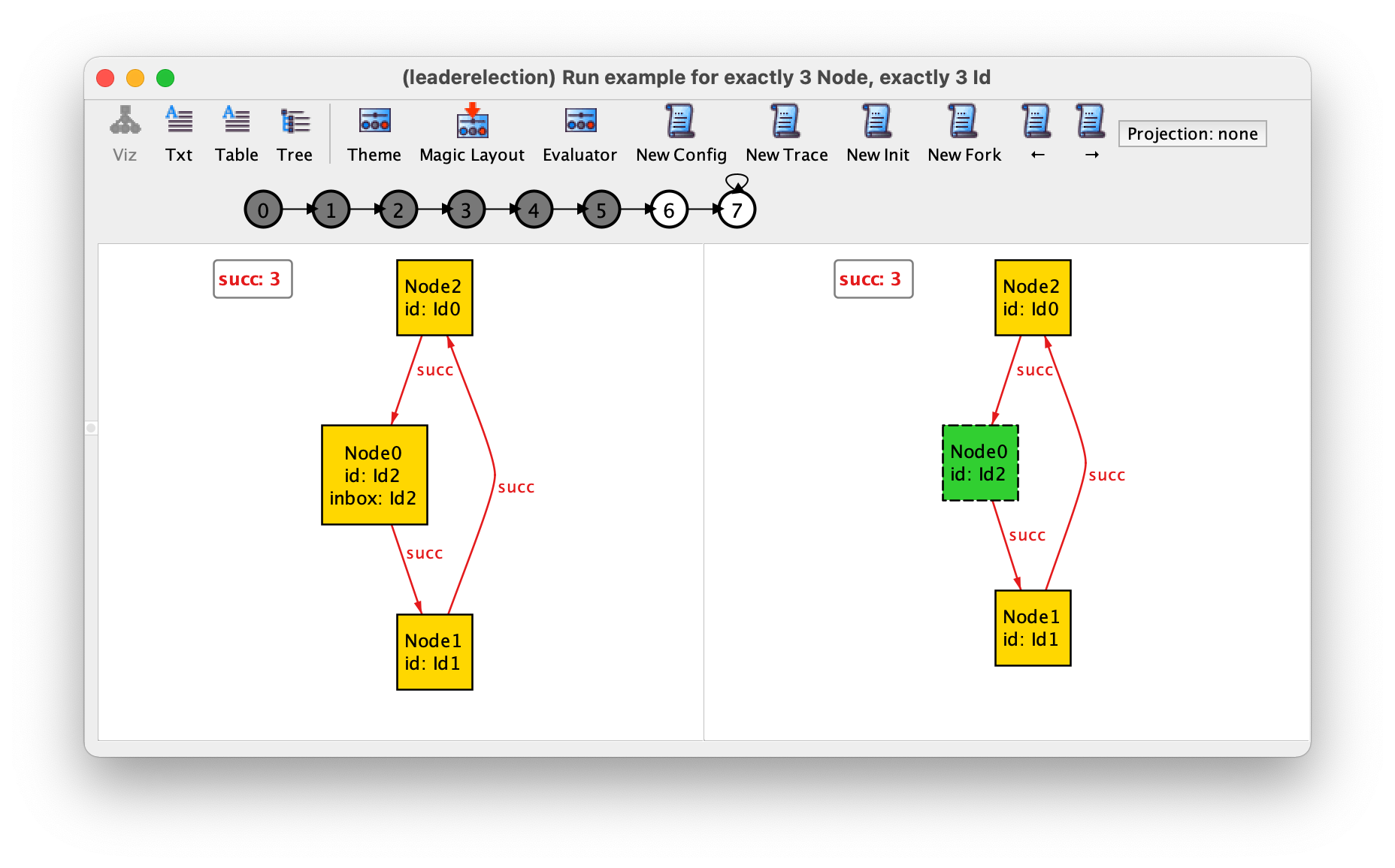
However, in the general case, for more complex specifications, the fact that events aren’t displayed makes their interpretation tedious and error-prone. The crux of the idiom presented here is to use derived relations to represent the events happening in a given state.
This may not seem immediately obvious as derived relations define relations based on existing signatures, while we haven’t got any such signature for events, only predicates. No problem! Let’s introduce a signature (more precisely: an enumeration, since the required atoms are known and we won’t need to add fields) representing event names. Observe how we use the capitalised names of predicates (corresponding to events) as elements of the enumeration, in order to enhance readability.
enum Event { Stutter, Initiate, Send, Process } // event names
Also, in the theme customisation menu, change the shape and colour of events, for instance to a red parallelogram. Then set Hide unconnected nodes to On for Event nodes, as we don’t want to see all event names at all states, but only those corresponding to events occurring in a given state.
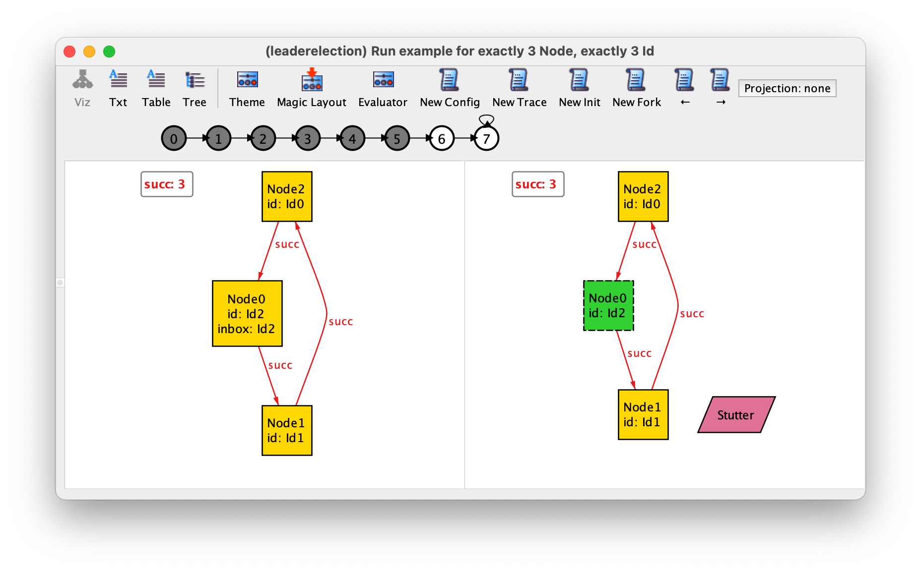
Now, let’s introduce a first derived relation, which should be populated when the stutter event happens. Recall that derived relations that refer to mutable elements are evaluated in the state they are being called from.
fun stutter_happens : set Event {
  { e: Stutter | stutter }
}
This definition may seem strange at first but this is indeed what we want: the stutter_happens derived relation yields, in every state, a subset of Event that will be populated (by the name Stutter) if the stutter predicate is true, and empty otherwise.
Observe the effect of adding this derived relation on visualisation. First, open the theme customisation menu and set both Hide unconnected nodes and Show as labels to Off for stutter_happens. This will override the hiding of Event nodes that belong to stutter_happens. Then head to the last states of the trace (where the stutter event happens). You will now be able to observe the event happening, as shown below.
Now, let’s consider the initiate event. This event takes a node as a parameter. In this case, the derived relation shouldn’t just yield the Initiate name as we wouldn’t be able to tell for which node or nodes it is satisfied. We rather return the set of all pairs whose first coordinate is the Initiate name and whose second coordinate is a node on which the initiate event happens:
fun initiate_happens : Event -> Node {
  { e: Initiate, n: Node | initiate[n] }
}
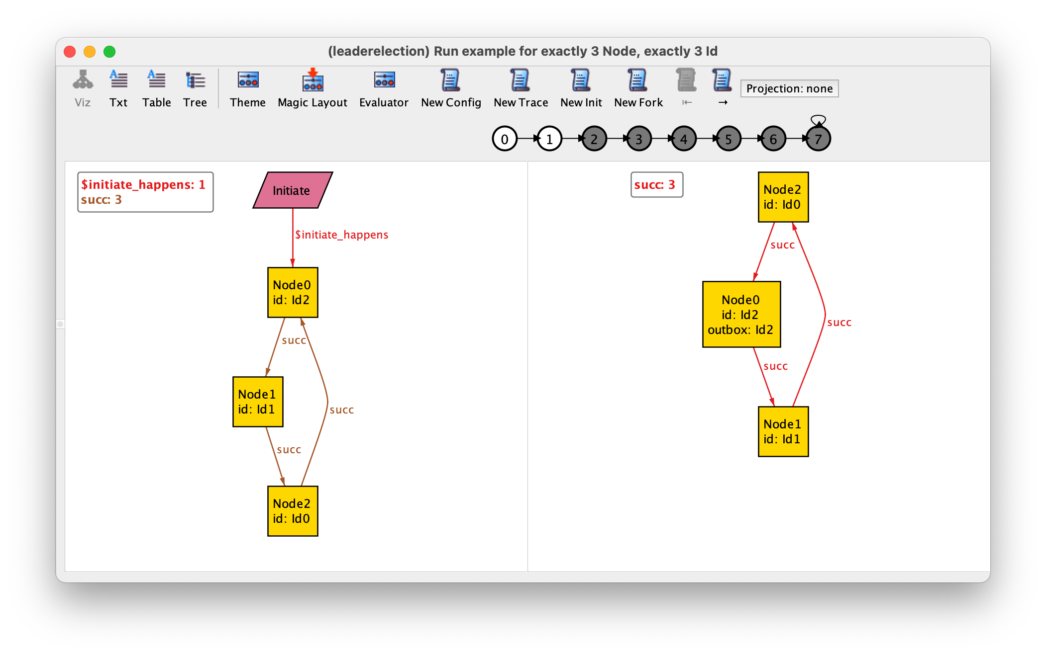
Now the first state of the trace is as follows. Since Event nodes
related by initiate_happens are no longer unconnected, they will show
up in the visualization without needing to change theme as was the case for
stutter_happens.
We can finally proceed with the last two events:
fun send_happens : Event -> Node -> Id {
  { e: Send, n: Node, i: Id | send[n, i] }
}

fun process_happens : Event -> Node -> Id {
  { e: Process, n: Node, i: Id | process[n, i] }
}
As you start visualising a trace, you may realise that the depiction of events without further theme customization is deficient when an event takes two parameters or more. A possible enhancement is to show event parameters as labels rather than edges. To do so, we can introduce a further derived relation that just returns the set of names of all occurring events.
fun events : set Event {
  stutter_happens + initiate_happens.Node + (send_happens + process_happens).Id.Node
}
Note that, for instance, expression initiate_happens.Node projects away any parameter of initiate events and keeps only the event name.
Then the following theme can be configured:
Uncheck Hide unconnected nodes for the
eventsset and set Show as labels to Off.In the relations part, set all derived relations for events to Show as attribute and change the displayed name for the derived relations to
args.
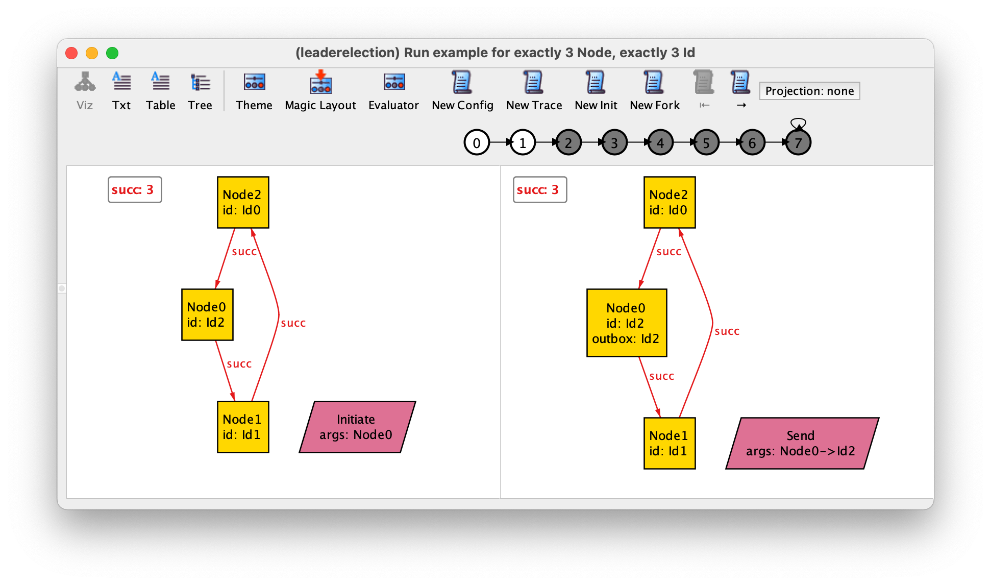
This way, we get the following depiction. Notice how the arguments of events can be seen clearly (e.g. Node0 and Id2 for the event send in state 1).
This is it for the idiom enabling a more informative depiction of traces!
At the beginning of this section, however, we also said that the idiom is useful to specify certain classes of formulas in a nice way. Let’s explore this aspect. First, the idiom allows to greatly simplify the traces fact!
fact traces {
  // possible events
  always some events
}
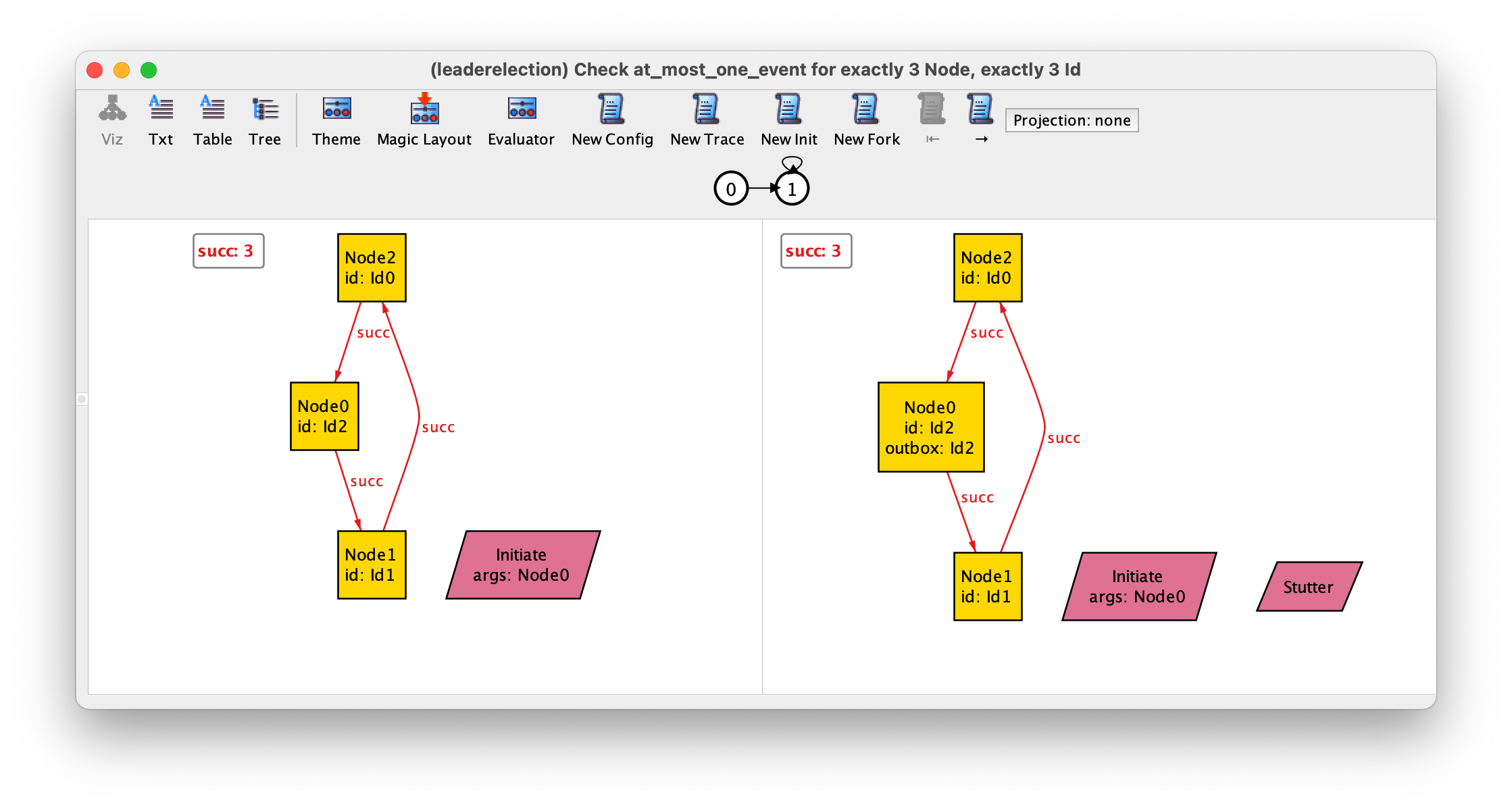
You may also check whether it is possible to witness the occurrence of two events in the same state, which happens to be the case.
check at_most_one_event {
  always lone events
} for exactly 3 Node, exactly 3 Id
However, if, for example, we remove the guard from event initiate this property yields the following counter-example, where an occurrence of initiate is undistinguishable from stuttering. This was an issue already explored back in chapter Protocol design with Alloy.
More importantly, notice that predicates and functions belong to different namespaces in Alloy. Additionally, they can always be disambiguated based on the syntactic context. For this reason, it is possible to give to the functions defined above the same name as the respective predicates!
fun stutter : set Event {
  { e: Stutter | stutter }
}

fun initiate : Event -> Node {
  { e: Initiate, n: Node | initiate[n] }
}

fun send : Event -> Node -> Id {
  { e: Send, n: Node, i: Id | send[n, i] }
}

fun process : Event -> Node -> Id {
  { e: Process, n: Node, i: Id | process[n, i] }
}

fun events : set Event {
  stutter + initiate.Node + (send + process).Id.Node
}
Now suppose you want to see the example of a trace in which two process events happen in a row (for some arguments). Until now, you would have had to write this in a rather contrived way, for instance as follows.
run two_process_in_a_row {
  eventually (
    (some n: Node, i: Id | process[n, i]) and
    after (some n: Node, i: Id | process[n, i])
  )
} for exactly 3 Node, exactly 3 Id
Yet, the derived relations defined above are also useful to say that an event happens (for some parameters). Indeed, it is enough to say that the corresponding derived relation is non-empty!
run two_process_in_a_row {
  eventually (some process and after some process)
} for exactly 3 Node, exactly 3 Id
Thus, giving the same name to a predicate (representing an event) and to the respective derived relations makes it easy to say that an event e happens: you just have to write some e!
As a final remark, notice that this idiom doesn’t entail any performance penalty:
If derived relations are only used for the depiction of events, they are only computed when visualising instances.
If they are also used in formulas, to say for instance that an event happens, they actually use less variables than the version where a predicate is passed arguments quantified existentially.
Thus, the only price to pay is a small but systematic inflation, albeit admittedly tedious, of our models. In the future, an extension to Alloy may be proposed to automate this task.
Using the evaluator to debug specifications
Chapter Structural design with Alloy has briefly introduced the evaluator provided
by the Analyzer. The evaluator, accessible through the Evaluator
button in toolbar of the instance visualiser, allows the user to evaluate any
formula or expression over the instance currently opened in the visualizer.
For instance, let us get back to the last example instance from the previous
section. The evaluator can be used to query simple elements of the model, like
signature Dir, field entries or function empty_dirs,
presenting their values for the current instance (the tuple set in tabular
style for an expression, true/false for a formula). But
perhaps more interesting, the evaluator is also able to interpret any valid
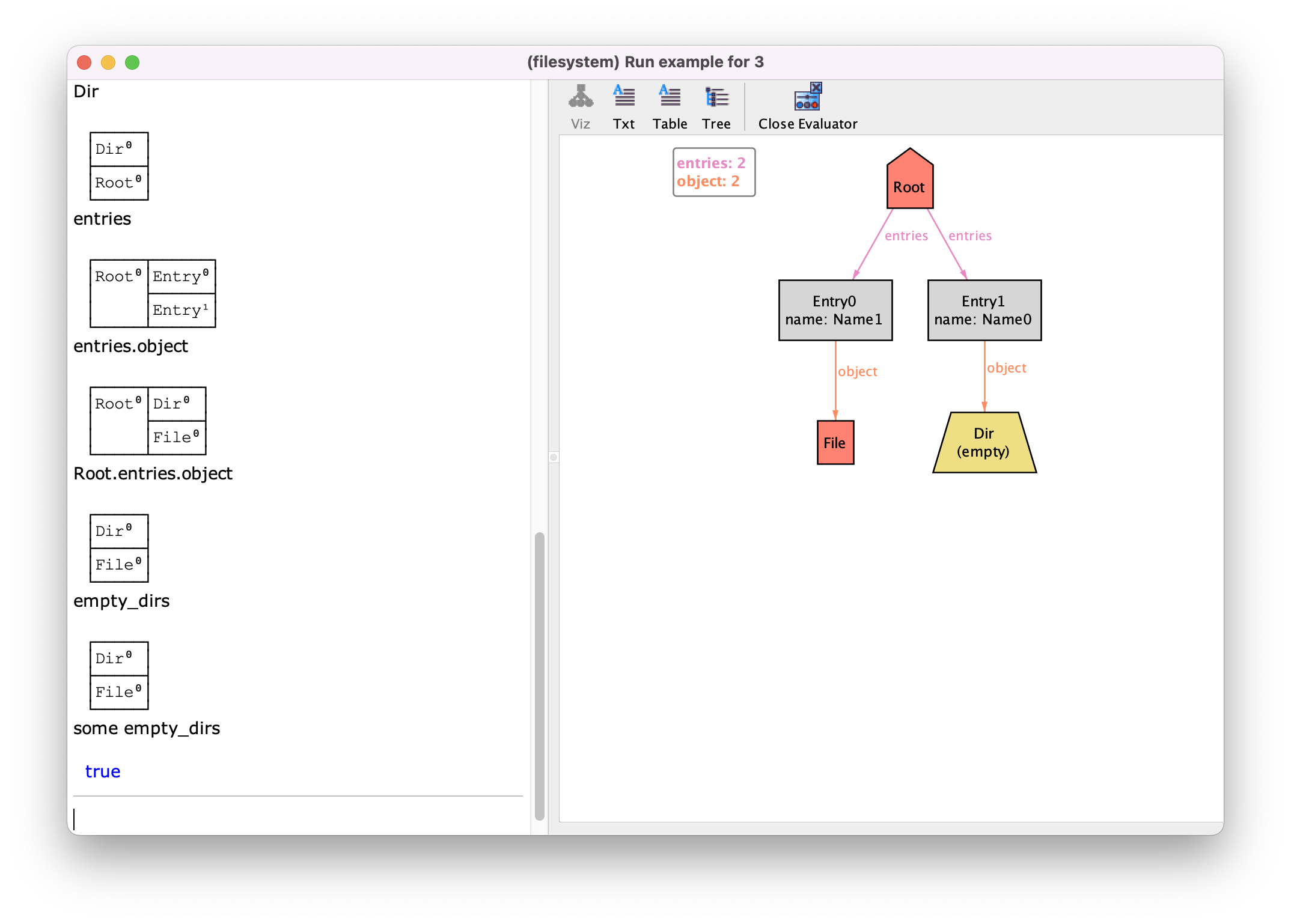
relational expression or formula. For instance, one may wish the content of
all directories by evaluating entries.object, or even apply it to the
concrete signature Root. Or one can query whether there is
some empty directory in the instance. The result is depicted as
follows. Note that you can navigate through the evaluator log with ↑
and ↓.
A feature of the evaluator that is particularly helpful when inspecting a
instance, is that unlike in the model specification, we can refer to concrete
atoms in the expressions passed to the evaluator. This is possible because
once a concrete instance is known, the universe of atoms is fixed. To refer to
a concrete atom, you should use the label of its most specific sub-signature
as the prefix and its numerical identifier as a suffix, separated by a
$ mark (except for Int and String atoms, which are
referred by their concrete values).. Note that subset signatures do not affect
the name of an atom (since each atom may belong to multiple subsets). Back to
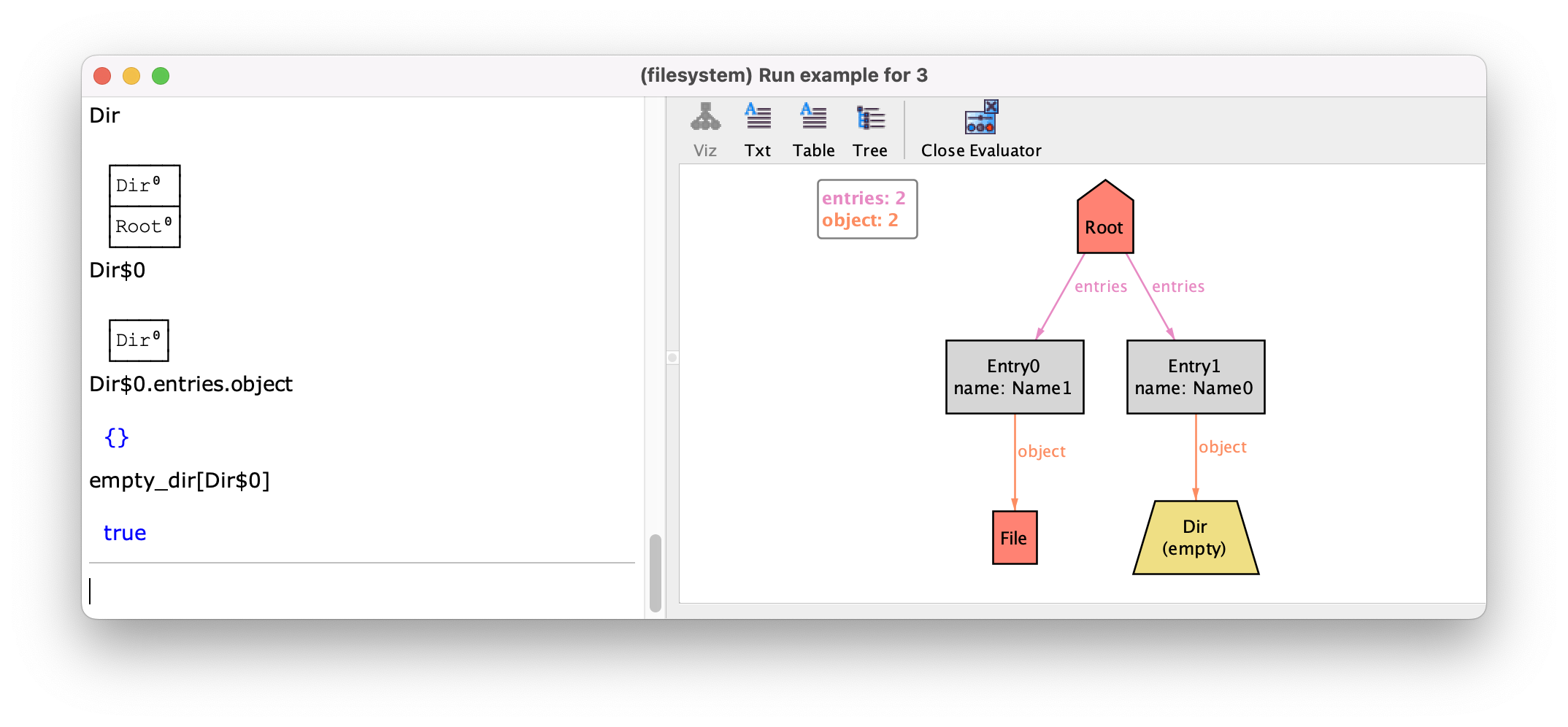
the example, you can for instance query the content of directory Dir$0
with Dir$0.entries.object (which happens to be empty). You can also
call model functions or predicates with atoms as arguments. For instance,
consider a predicate that tests whether a given directory is empty:
pred empty_dir[d:Dir] {
  d in empty_dirs
}
You could now simply call empty_dir[Dir$0] in the evaluator. The
result is shown below.
Note
Atom name mismatch.
You may have noticed some differences between the atom names in calls to the
evaluator and their representation in the evaluator response and in the
visualizer, namely the absence of the $ mark. That’s because the
some pretty printing is employed to ease readability, but the evaluator must
be able to distinguish an atom A$0 from a model signature A0
(recall that signature names are alpha-numerical).
Note also that any theme customization applies only to the graph view, and not to the evaluator. This means that, for instance, if you change the label of a signature or relation in the theme, the evaluator will still only recognize and print the original label. If this gets confusion, you can always temporarily tick the option Use original atom names in the theme customizer.
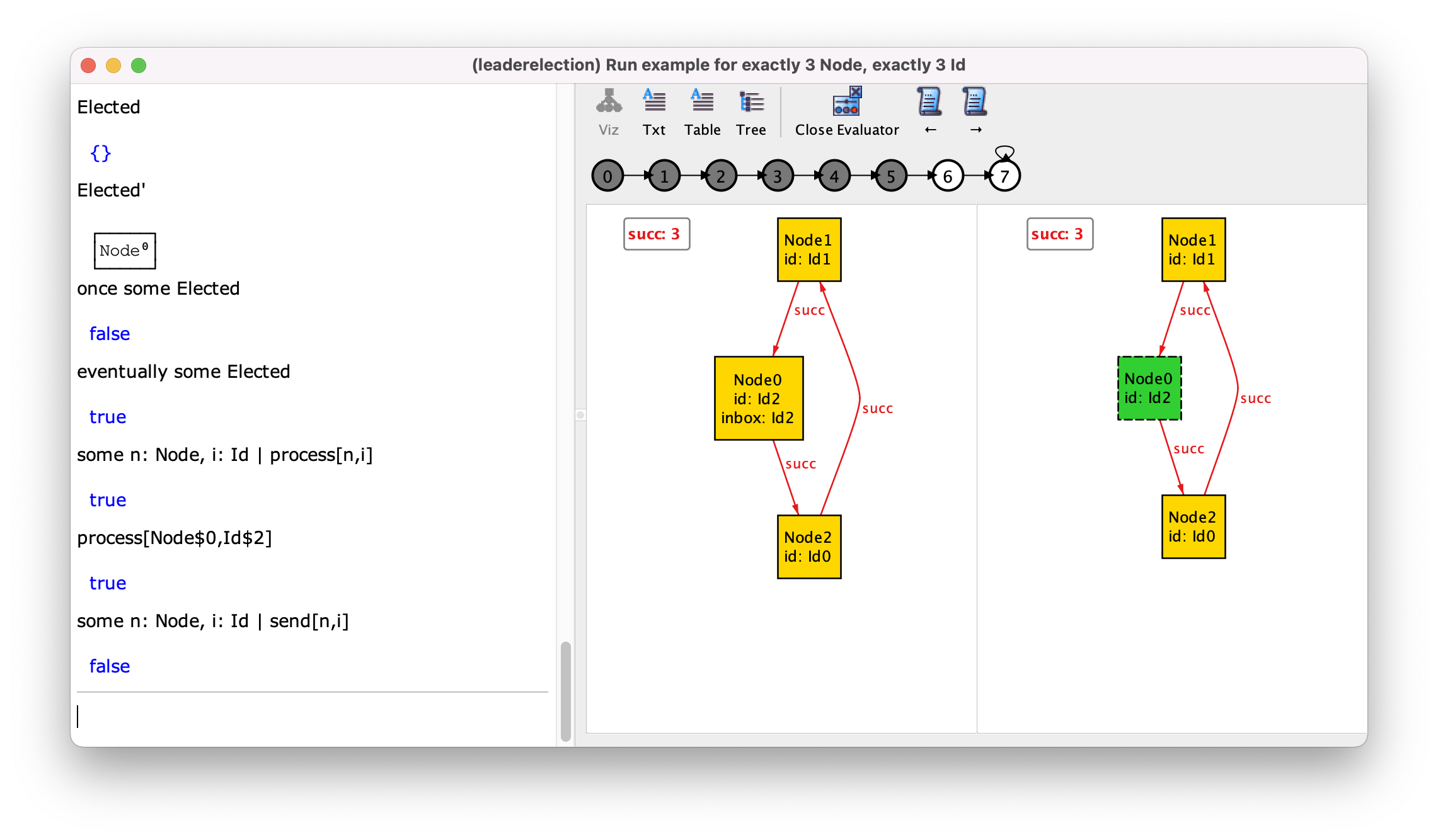
If the instance under analysis is a trace, temporal expressions and formulas
can be freely used, and are evaluated from the currently focused state (the
one at the left-hand side of visualization). For instance, consider an
example trace from chapter Protocol design with Alloy where a leader is
eventually elected at the 8th state. Focusing on the 7th state, as shown
below, one can inspect how the state changed between those two states. For
instance, calling Elected and Elected' will show that a node
has been elected leader. We can also evaluate temporal formulas, in this case
testing whether there had been any leader in the past, or whether there will
be some in the future (false and true, respectively, as expected). Another
interesting use of the evaluator is to understand which event has happened
between two states. As explained in Protocol design with Alloy, since events are
just regular predicates they are not depicted in the instance, and the next
section will precisely present an idiom to visually depict the occurring
events. However, you can also just call the event predicates from the
evaluator and test their occurrence, including with concrete atom as
arguments.
As a last note, it is worth mentioning that evaluation over a specific instance is very efficient, so it can be used regularly.
Defining test scenarios with formulas
As an Alloy specification increases in size and complexity, its validation
through the exploration of arbitrary instances in the visualizer becomes less
useful, since getting varied instances is increasingly unlikely. This is even
more patent when exploring trace instances, despite the exploration operations
provided by the visualizer. At that point, one must combine this exploration
with the specification of finer run commands. Note that often we don’t want
the command completely fix the instances since we want to be able to explore
the design. Instead, we want to partially specify interesting scenarios that
the Analyzer will complete by solving the specification’s constraints. This is
not necessarily trivial for complex specifications.
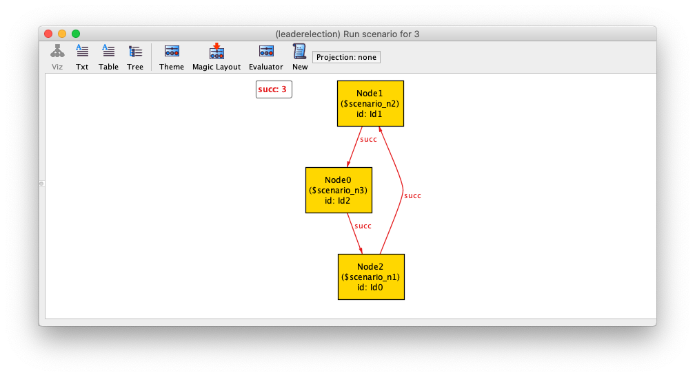
This first issue we often face is the inability to refer to concrete atoms in Alloy specifications. Let’s start with the specification of scenarios for instances without mutable signatures and fields, on which we will later build to specify trace scenarios. Let’s consider the structural part of the leader election example from chapter Protocol design with Alloy and say that we want to explore scenarios with 3 nodes with sequential identifiers.
We can achieve through an idiom based on some/disj patterns.
For instance, the scenario above could be defined as follows.
run scenario {
  some disj n1, n2, n3 : Node, i1, i2, i3 : Id {
    Node = n1 + n2 + n3
    Id   = i1 + i2 + i3
    next = i1 -> i2 + i2 -> i3
    succ = n1 -> n2 + n2 -> n3 + n3 -> n1
    id   = n1 -> i1 + n2 -> i2 + n3 -> i3
  }
} for 3
The disj keyword is needed in order to avoid the assignment of the
same atom to different variables. For instance, without disj here a
single node atom assigned to n1, n2 and n3, pointing
to itself, would be a valid instance. Moreover, the equality test with
Node guarantees that no other atom will exist in Node besides
the 3 quantified. The subsequent lines enforce the value of the fields to
define the desired ring topology. Always make sure that there are enough
atoms in the scope to represent the scenario, otherwise the command will
be trivially unsatisfiable.
Due to the mechanics explained in section Improved visualisation with derived relations, the quantified
variables appear identified in the visualizer, prefixed by a $ and the
name of the command, as shown below. This can be customized in the theme.
Note that, as with anything Alloy, these specifications can be mixed with other constraints. For instance, the same scenario, where identifiers are sequential, could be equally specified as follows.
run scenario {
  some disj n1, n2, n3 : Node, i1, i2, i3 : Id {
    Node = n1 + n2 + n3
    Id   = i1 + i2 + i3

    all n : Node | n.id.(next + last -> first) = n.succ.id
  }
} for 3
As run commands become more restricted, they become less interesting for
validation, since the room for unpredictable results is reduced. However,
these commands also serve a second purpose: they can be used as a kind of
regression testing, commands that we know must hold (or fail) for our
specification, and that can be re-executed whenever the specification evolves.
Alloy has an expects keyword for commands that can help managing these
commands.
Note
What about multiplicity one signatures?
At first sight, one could declare 3 pairs of signatures with multiplicity
one extending Node and Id to specify all the atoms
we need, and then call those signatures in run commands. However, this
approach has a major disadvantage: introducing such signatures in the
specification affects all analysis commands in the specification. For
instance, all check commands would only consider instances
where there were at least 3 nodes. Perhaps even worse, it would break
the symmetry between those atoms, as they would no longer be
uninterpreted, and isomorphic instances would be returned. Unless we are
dealing with concepts of the domain model, we should not clutter our
specifications with additional signatures. The some/disj
pattern provides a way to specify scenarios that is local to each
command.
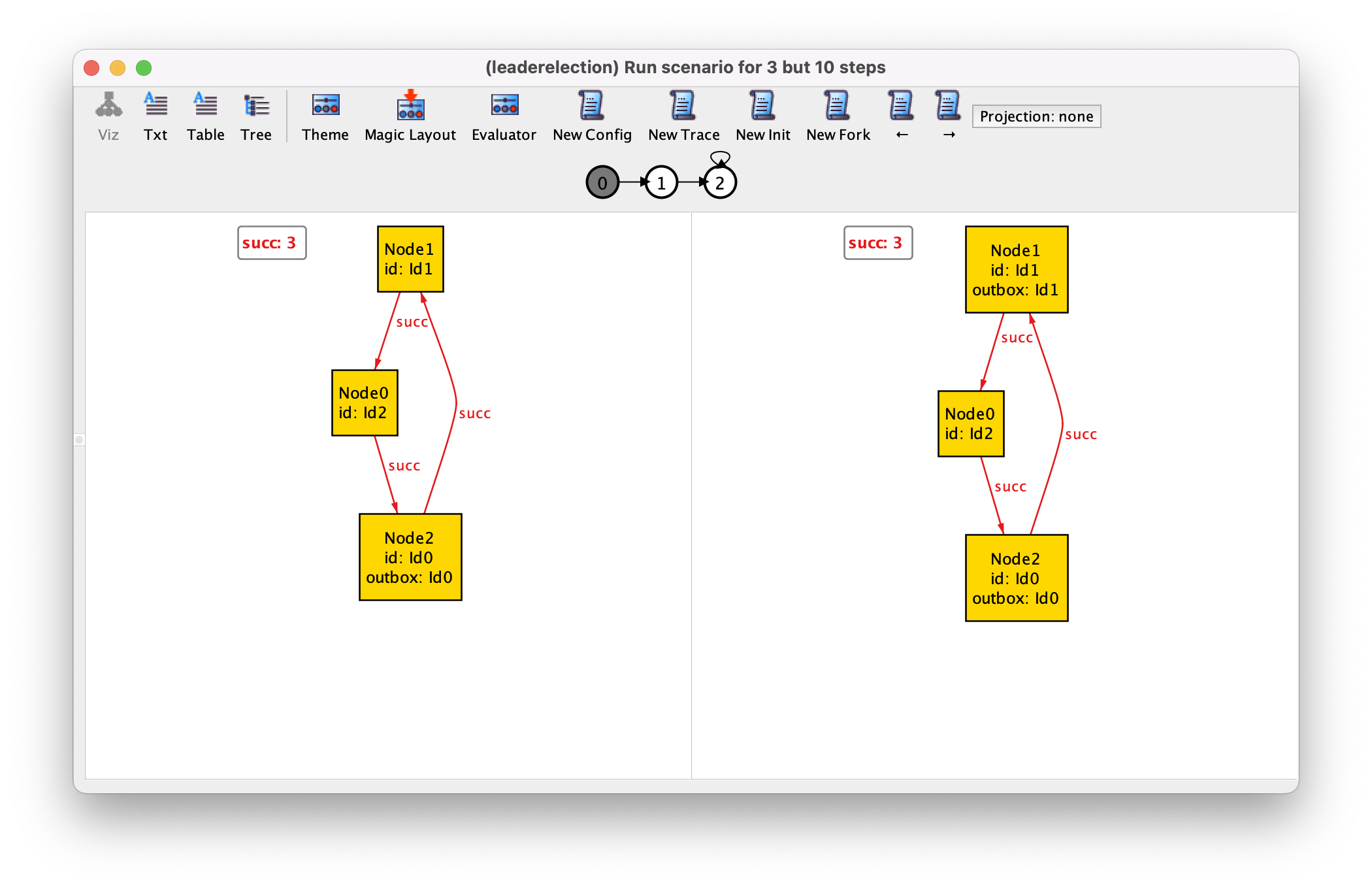
Moving to the mutable context, we must now extend such formulas to restrict
multiple states. The main issue here is that with the temporal operators we
have seen so far, this would result in either nested and/after
formulas, or expressions with several appended primes ', neither being
a scalable approach. Luckily, Alloy has a sequential temporal operator
; that greatly eases specifying such formulas. For instance, the code
below restricts the value of inboxes and outboxes in the first 3 states.
run scenario {
  some disj n1, n2, n3 : Node, i1, i2, i3 : Id {
    Node = n1 + n2 + n3
    Id   = i1 + i2 + i3
    next = i1 -> i2 + i2 -> i3
    succ = n1 -> n2 + n2 -> n3 + n3 -> n1
    id   = n1 -> i1 + n2 -> i2 + n3 -> i3

    no outbox; outbox = n1 -> i1; outbox = n1 -> i1 + n2 -> i2
    no inbox;  no inbox;          no inbox
  }
} for 3 but 10 steps
Again, we can leave these formulas as underspecified as we wish. For instance,
we are not restricting the value of Elected, which will be solved
during analysis. Moreover, by restricting only 3 states, the succeeding ones
will be freely solved by the Analyzer. Again, make sure that there are steps
in the scope to represent the scenario. Alternatively, one could enforce a
final state forbidding any further changes with a temporal always as
follows.
run scenario {
  some disj n1, n2, n3 : Node, i1, i2, i3 : Id {
    Node = n1 + n2 + n3
    Id   = i1 + i2 + i3
    next = i1 -> i2 + i2 -> i3
    succ = n1 -> n2 + n2 -> n3 + n3 -> n1
    id   = n1 -> i1 + n2 -> i2 + n3 -> i3

    no outbox; outbox = n1 -> i1; always outbox = n1 -> i1 + n2 -> i2
    no inbox;  no inbox;          always no inbox
  }
} for 3 but 10 steps
In fact, all formulas inside the sequence can also be temporal, but they become difficult to manage outside this pattern.
The example above followed a relation-wise definition of the trace. Sometimes, however, it’s easier to think about scenarios state-wise, particularly for relations closely related. Following this idiom, this could also be achieved as follows.
run scenario {
  some disj n1, n2, n3 : Node, i1, i2, i3 : Id {
    Node = n1 + n2 + n3
    Id   = i1 + i2 + i3
    next = i1 -> i2 + i2 -> i3
    succ = n1 -> n2 + n2 -> n3 + n3 -> n1
    id   = n1 -> i1 + n2 -> i2 + n3 -> i3

    no outbox + inbox;
    outbox = n1 -> i1 and no inbox;
    always (outbox = n1 -> i1 + n2 -> i2 and no inbox)
  }
} for 3 but 10 steps
As a last tip, sometimes we end up defining multiple scenario commands that share a certain part of the specification. At this point it is often useful to refactor-out parts of the specification into derived predicates. For instance, if we wanted to define multiple scenarios for the same ring topology:
pred seq_ring [n1, n2, n3 : Node, i1, i2, i3 : Id] {
  Node = n1 + n2 + n3
  Id   = i1 + i2 + i3
  next = i1 -> i2 + i2 -> i3
  succ = n1 -> n2 + n2 -> n3 + n3 -> n1
  id   = n1 -> i1 + n2 -> i2 + n3 -> i3
}

run scenario {
  some disj n1, n2, n3 : Node, i1, i2, i3 : Id {
    seq_ring[n1,n2,n3,i1,i2,i3]

    no outbox + inbox;
    outbox = n1 -> i1 and inbox = n1 -> i1;
    always (outbox = n1 -> i1 + n2 -> i2 and inbox = n1 -> i1 + n2 -> i2)
  }
} for 3 but 10 steps