Protocol design with Alloy
In this chapter we will explain how to specify and analyse a distributed protocol using Alloy. We will use a very simple example of a leader election protocol. The aim of a leader election protocol is to designate one node in a network as the organizer or leader of some distributed task. Nodes are initially unaware of which node will play that role, but after running the protocol all nodes should recognise the same node as leader. Many different leader election protocols exist: here we will use a well-known version that can be used to elect a leader in a network of nodes organised in a ring, and where nodes also have unique identifiers. This is an example commonly used when presenting idioms for behaviour specification in Alloy [MIT12]. This protocol was proposed by Chang and Roberts [CACM79] and roughly operates as follows: the goal is to elect as leader the node with the highest identifier; each node starts by sending its own identifier clockwise; upon receiving an identifier, a node only forwards it if it is higher than its own; a node receiving back its own identifier designates itself as leader; finally the leader broadcasts its newly found role to the network. In our specification we will not model this last (trivial) step, and will only be concerned with the fundamental property of a leader election protocol: eventually exactly one (exactly one) node will designate itself as the leader.
Specifying the network configuration
When designing a distributed protocol, we should start by specifying the network configurations in which it is supposed to operate. In this case, the protocol operates in a ring network of nodes with unique identifiers. Notice that many different network configurations satisfy this requirement: we could have rings of different size, and for the same size, different assignments of the unique identifiers to the nodes (the relevant fact here is the relative order in which the identifiers appear in the network). The verification of the expected properties of the protocol should take into account all possible different configurations (up to the specified bound on the ring size). The network configuration, although arbitrary, does not change during the execution of the protocol. As such, it will be specified with immutable sets and relations.
Unlike some formal specification languages, Alloy has no pre-defined notion of process or node. These have to be explicitly specified, by declaring a signature. Since the network of nodes forms a ring, a binary relation that associates each node with its immediate successor in the ring should also be declared.
sig Node {
  succ : one Node
}
Recall that binary relations should be declared as fields inside the
domain signature. In the declaration of field succ the
multiplicity one is used to ensure that each node has exactly
one successor in the ring. As usual in Alloy, we can immediately start
validating our specification by asking for example instances using a
run command.
run example {}
By iterating over the returned instances with New we could get the following instance, which is not a valid ring.
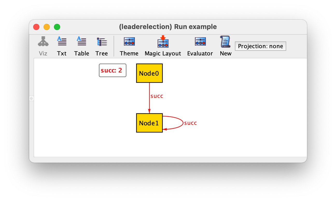
In addition to requiring each node to have exactly one successor, a simple way to ensure that a network forms a ring is to require that
every node is reachable from any other node. Given a node n,
to determine the set of nodes reachable from n via relation
succ we can use expression
n.^succ. This expression makes use of the composition (.) and transitive closure (^) operators already presented in chapter Structural design with Alloy. The constraint that succ forms a ring can thus be specified in a fact as follows.
fact {
  // succ forms a ring
  all n,m : Node | m in n.^succ
}
An alternative specification is to require that the set of all nodes
(denoted by Node) is reachable from every node.
fact {
  // succ forms a ring
  all n : Node | Node in n.^succ
}
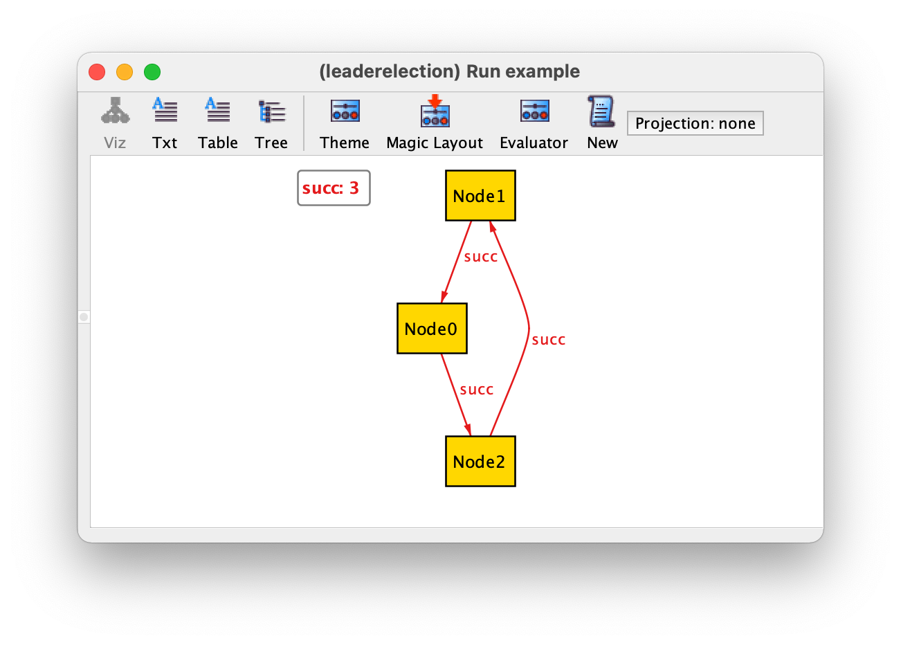
If we now iterate over all instances returned by command example we will get the 3 possible rings with up to 3 nodes and a configuration without any node, which is also allowed by our specification. The limit of 3 is due to the implicit command scope of 3 atoms per top-level signature. As an example we show the ring with 3 nodes.
To enforce that we have at least one node we can add the following fact.
fact {
  // at least one node
  some Node
}
Besides being organised in a ring, nodes must also have unique identifiers. Since we are going to need to compare identifiers, one possibility would be to just use integers to represent them. However, besides being totally ordered, integers carry additional semantics that is not necessary here. In particular, integers support arithmetic operations that will not be required in this example. When developing a formal specification it is good practice to be as abstract as possible, in particular avoid adding unnecessary restrictions. Also, the analysis of Alloy specifications with integers has some subtleties which makes it better to avoid, unless strictly necessary (see Working with integers for a proper discussion). As such, we will introduce a signature Id, to denote identifiers, and a binary relation next to capture the total order between them.
sig Id {
  next : lone Id
}
Given an identifier, relation next shall yield the next identifier in the total order. All identifiers except the last one have a next, so the multiplicity of this relation should be lone.
To constrain next to entail a total order over Id we could, for example, declare singleton signatures to denote the first and last identifiers, require the last to have no next, and all identifiers to be reachable from the first via the (reflexive) transitive closure of next.
one sig first, last in Id {}

fact {
  // Id is totally ordered with next
  no last.next
  Id in first.*next
}
Here we used in instead of extends to declare the singleton sets first and last. Recall that extension signatures are disjoint, while inclusion signatures are arbitrary subsets of the parent signature. In this case we what the latter because when we have just a single Id, first and last should be the same identifier. In the last constraint we used operator * to compute the reflexive transitive closure of next, to get all identifiers that are reachable in zero or more steps via next (the transitive closure would yield all identifiers reachable in one or more steps). The reflexive transitive closure is defined as *next = ^next + iden, the union of the transitive closure and the predefined identify binary relation, that relates each element of our universe of discourse to itself.
Warning
Understanding the predefined Alloy constants.
There are three predefined (relational) constants in Alloy:
none, that denotes the empty set.univ, the set of all atoms in all signatures.iden, the binary relation that associates each atom inunivto itself.
It is important to know that when there are mutable top-level
signatures (declared with var), both univ and
iden are mutable also, with the former containing, in each
state, all atoms contained in all signatures at that state.
It is also important to remember that iden relates every element of univ to itself. This means that, for example, to check that a binary relation R (defined on a signature A) is reflexive it is not correct to write iden in R, as iden will not only contain elements in A but also elements in other declared top-level signatures. To obtain the identity relation on signature A we could, for example, intersect it with the binary relation containing all pairs of elements drawn from A, computed with the Cartesian product operator ->, as follows: iden & (A -> A). Alloy also has an operator to restrict the domain of a relation that can be used for the same effect: A <: iden filters relation iden to obtain only the pairs whose first element belongs to A. Dually, we could have restricted the range: iden :> A filters relation iden to obtain only the pairs whose last element belongs to A. Thus, to check that the relation R is reflexive we could write, for example, (A <: iden) in R.
Another thing to recall is that none denotes the empty set and is a unary relation. So, if we write R = none, to check if R is empty, we will get a type error since the relations have different arities (none is unary and R is binary). The empty binary relation is denoted by the Cartesian product none -> none: this expression denotes the empty set like none, but for the type system it is a binary relation, so writing R = (none -> none) does not raise a type error. Of course, a simpler way to check that R is empty is to write no R: the cardinality check keywords like no can be used with relational expressions of arbitrary arity.
Having our identifiers totally ordered, we can now declare a field id inside signature Node, to associate each node with its identifier.
sig Node {
  succ : one Node,
  id : one Id
}
To ensure that identifiers are unique it suffices to require id to be injective, which can be done as follows.
fact {
  // ids are unique
  all i : Id | lone id.i
}
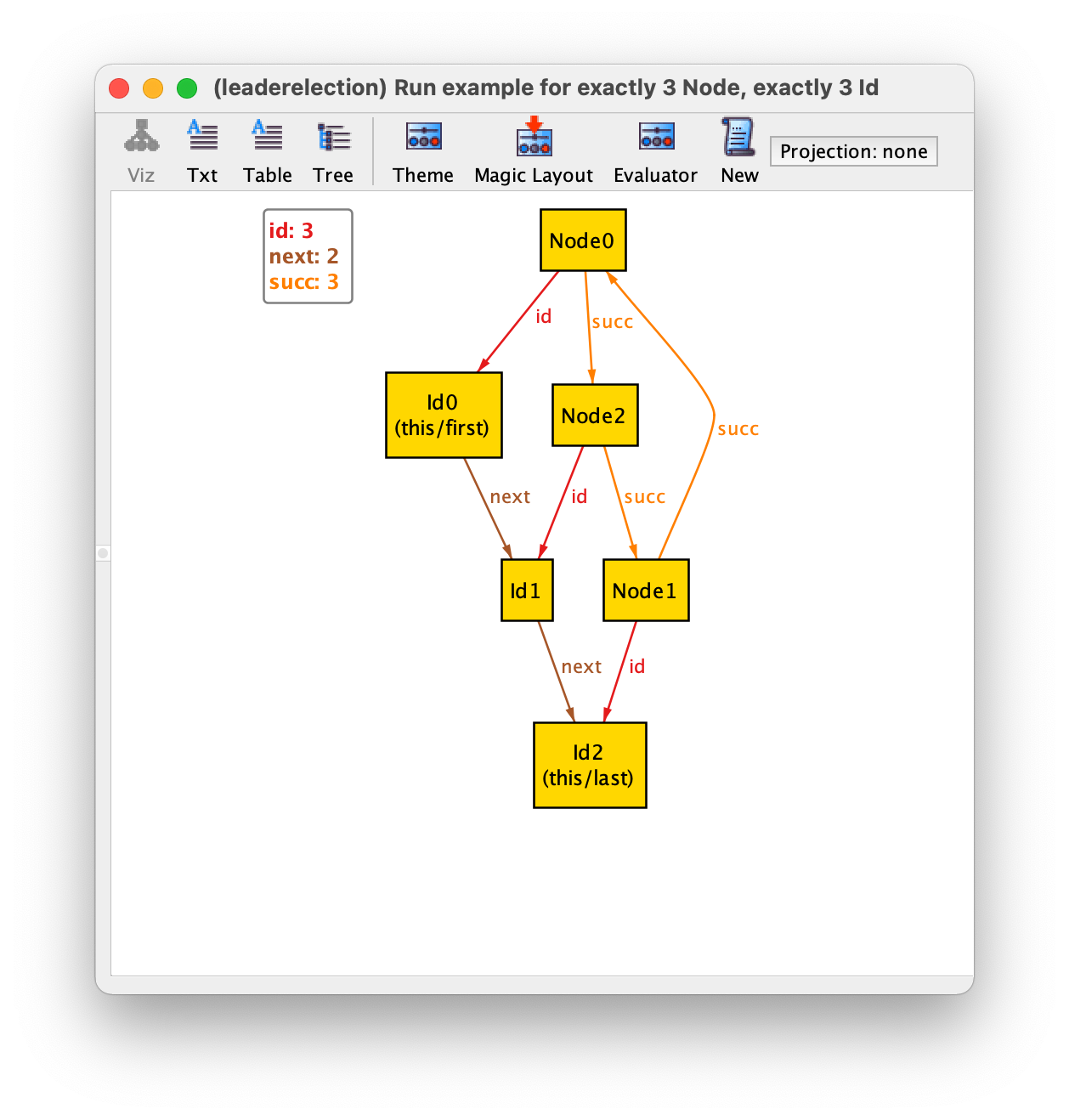
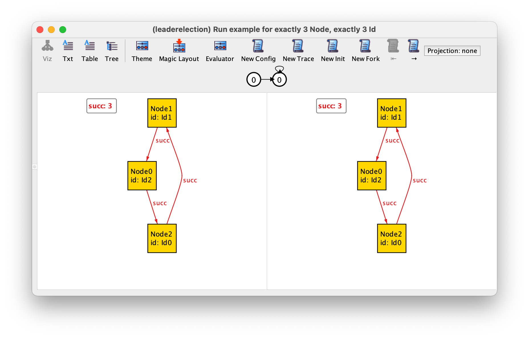
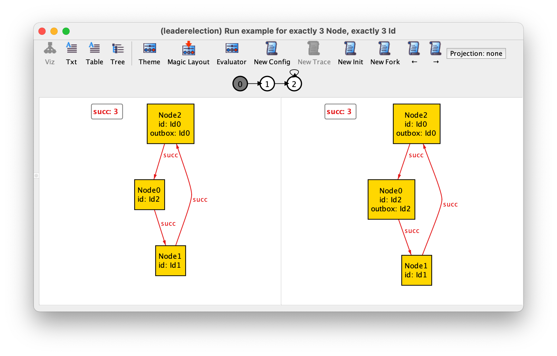
If we change the example command to ask for all configurations with exactly 3 nodes and 3 identifiers
run example {} for exactly 3 Node, exactly 3 Id
and iterate over all instances with New, we will get the two only (truly) different configurations with this size: one where the identifiers increase as we move clockwise in the ring, and another where they decrease. The former is depicted below. This illustrates the power of Alloy’s symmetry breaking, which in this case prevents the return of any other instance (that necessarily would be isomorphic to one of these two).
Using modules to structure a specification
Requiring a signature to be totally ordered is quite common. To simplify the specification of such common patterns, and also to enable breaking a large specification into more manageable pieces, Alloy supports the concept of module, which behaves similarly to modules in other specification and programming languages. It is possible to create a module with some definitions and then import it in another module. For example we could define a module for totally ordered identifiers as follows.
module orderedids

sig Id {
  next : lone Id
}
one sig first, last in Id {}

fact {
  // Id is totally ordered with next
  no last.next
  Id in first.*next
}
The first line in a module consists of the keyword module
followed by the module name. Module names should match the path of the
respective file, so we should save it the with name orderedids.als and be in the same directory as the module that will import it. Having factored out these declarations into module orderedids,
we can now delete them from our main module, and instead import this new module by adding the following open statement at the beginning of the specification.
open orderedids
Module orderedids is not ideal, since it commits to a specific signature name to be totally ordered. To make it more reusable, we could instead parametrise it by the signature one wishes to be totally ordered. This poses a problem, because our formalisation of a total order requires declaring field next inside the signature to be totally ordered, and modules cannot change the definition of the parameter signature. There are some tricks to solve this problem. One possibility is to declare an auxiliary inclusion signature inside the parameter signature, force it to be exactly the same as the parent signature using a fact, and declare relation next inside that auxiliary signature instead. The definition of our parametrised module (now called just ordered) would look as follows.
module ordered[A]

sig Aux in A {
  next : lone Aux
}
fact {
  Aux = A
}
one sig first, last in A {}

fact {
  // A is totally ordered with next
  no last.next
  A in first.*next
}
To use this parametrised module, we should declare back signature Id in our main specification, and pass it as a parameter in the open statement. The main specification should now look as follows.
open ordered[Id]

sig Node {
  succ : one Node,
  id : one Id
}

sig Id {}

fact {
  // at least one node
  some Node
}

fact {
  // succ forms a ring
  all n : Node | Node in n.^succ
}

fact {
  // ids are unique
  all i : Id | lone id.i
}

run example {} for exactly 3 Node, exactly 3 Id
Alloy has some predefined modules in a special util namespace. One of them is util/ordering, a parametrised module that behaves similarly to our module ordered, imposing a total order on a signature passed as parameter. This means that instead of defining our ordered module we could simply import this module with the statement
open util/ordering[Id]
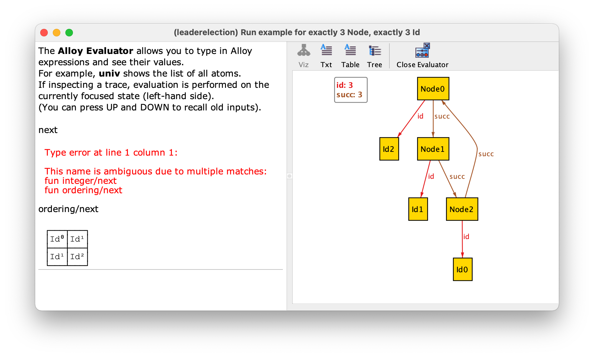
This predefined module is specified in a slightly different way but, as ordered, it exposes singleton sets first and last and a binary relation next that defines the total order. However, if we run the example command we get the following result.
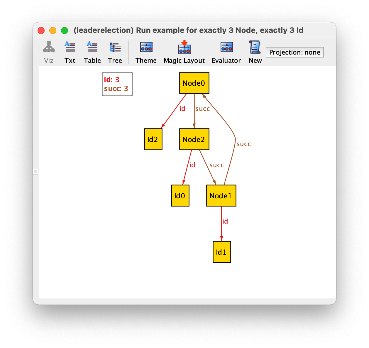
Due to the way they are defined in util/ordering, relations first, last, and next are not shown in the visualizer. In principle, this would make it very difficult to understand how the identifiers are ordered, but module util/ordering is handled in special way be the Alloy Analyzer, which will attempt to name the inhabitants of the ordered signature sequentially according to the order defined by next. In our instance this means that Id0 is the first, which is followed by Id1, and then Id2, which is the last. If we really want to confirm the value of the next relation we could go to the evaluator and ask for its value. However, we will get an ambiguity error since next is also defined in an integer module that is imported by default. To disambiguate we could type the qualified name ordering/next instead.
To see what other functions and derived relations are declared in util/ordering you can open it in the menu . For example, we have functions gt and lt to check if one element is greater than or less than another, respectively, and relation prev that returns the predecessor of an element, if it exists.
Warning
Be aware of exact scopes with util/ordering!
Besides naming the atoms according to the total order, module util/ordering has another peculiarity concerning the analysis. The scope of the signature that is passed as parameter to util/ordering is always exact even if not declared with exactly. This makes analysis faster but one should always be aware of this when running commands, as it may cause run commands to be trivially unsatisfiable and check commands to trivially have no counter-examples.
Consider the following specification, where we have model a finite set of natural numbers, distinguish between even and odd numbers, and require the first to be even and the last to be odd.
open util/ordering[Nat]

abstract sig Nat {}
sig Even, Odd extends Nat {}

fact {
  all n : Even | n.next in Odd
  all n : Odd | n.next in Even
  first in Even
  last in Odd
}

run example {}
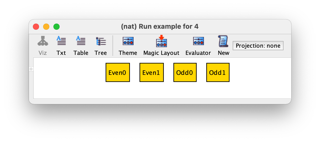
If we execute the command example we get no instance! This is due to the fact that the default scope for Nat is 3, and since it is being totally ordered with util/ordering this scope is required to be exact. Unfortunately, with exactly 3 atoms in Nat it is impossible to satisfy the given constraints. If we change the scope of example to 4 then we will obtain one instance.
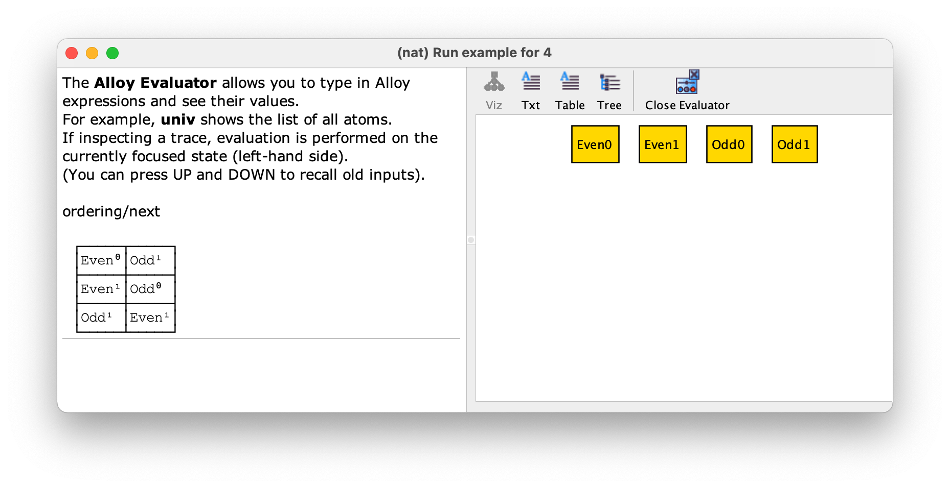
This is an example where the naming of the atoms does not help in understanding what is the total order, since the ordered signature Nat is abstract and extended by Even and Odd. By using the evaluator we can see that the total order is Even0, Odd1, Even1, and lastly Odd0.
As a last note on scopes, for efficiency reasons the util/ordering module also requires the parameter signature to be non-empty (since it forces first and last to always be defined), meaning that setting its scope to 0 results in an inconsistent specification.
Specifying the protocol dynamics
The coordination between the different nodes in this distributed protocol, like in many others, is achieved by means of message passing. Like nodes, Alloy has no special support for message passing, so all the relevant concepts have to be specified from scratch. In this case messages are just node identifiers, so there is no need to add a signature to model those. To capture the incoming and outgoing messages we can declare mutable binary fields inside signature Node, to associate each node with the set of identifiers it has received or that need to be sent, respectively. To declare a mutable field the keyword var should be used.
sig Node {
  succ : one Node,
  id : one Id,
  var inbox : set Id,
  var outbox : set Id
}
We also need to capture the nodes that have been elected as leaders. To do so we can declare a mutable signature Elected that is a subset of Node.
var sig Elected in Node {}
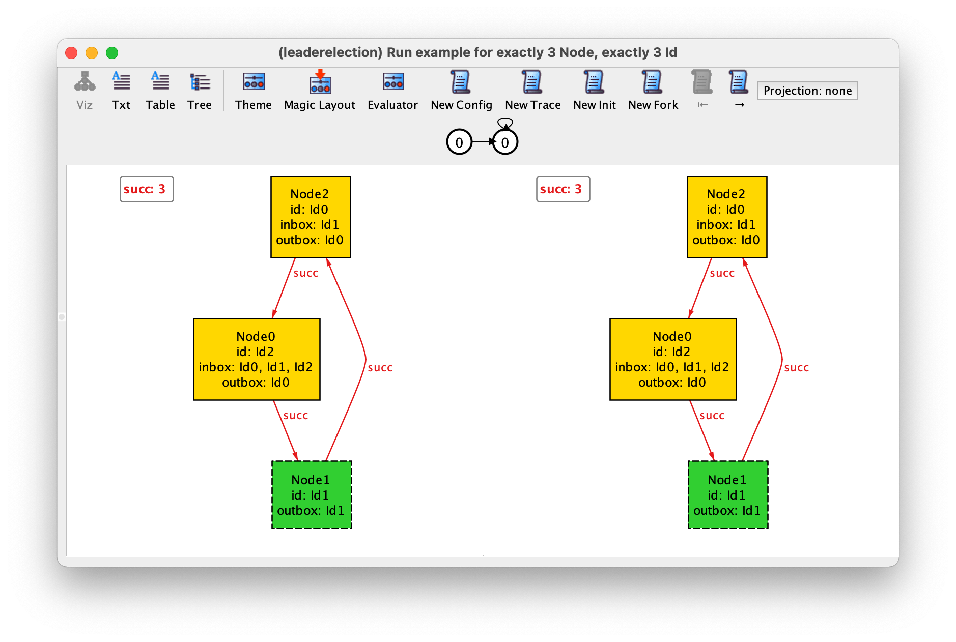
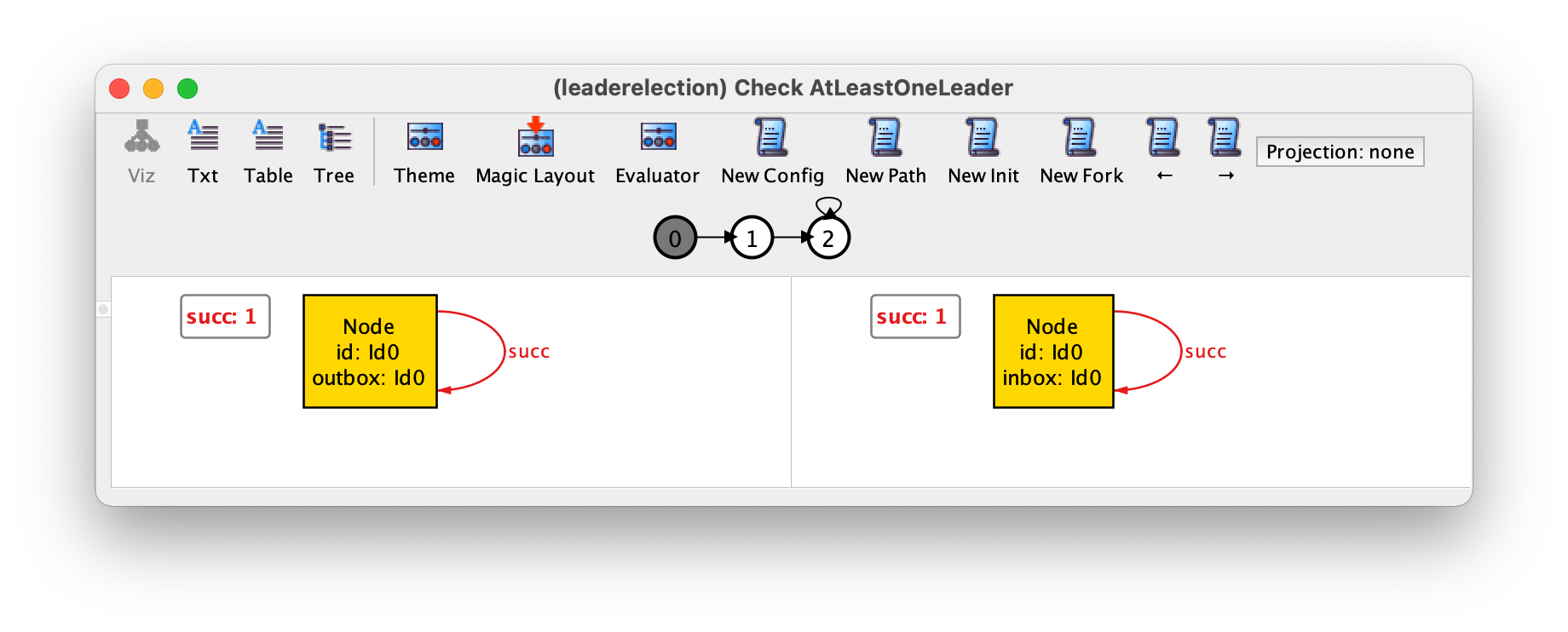
If we now run the example command we might get the following instance.
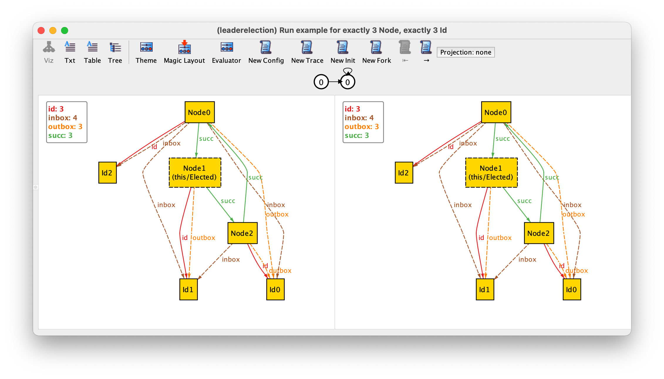
Once a specification has mutable elements, its instances take the shape of traces. The first thing to be noticed is that the interface of the visualizer changed to adapt to this fact: it now shows two instance snapshots side-by-side, there are several new instance exploration buttons in the toolbar, and a depiction of a path just below those. This new interface is due to the addition of mutable relations in our specification. As expected, the value of a mutable relation may change over time, so an instance of our specification can no longer be captured by a single static valuation of the declared signatures and fields. Instead, instances are now infinite sequences of states (aka paths or traces), being each state a (possibly different) valuation for the declared signatures and fields. As such, the visualizer now shows a (finite) depiction of the (infinite) trace, numbering the different states, and including a loop back that marks a segment of the trace that will repeat indefinitely. In this case we have a trace where the same state 0 repeats itself indefinitely, something that is possible since so far we added no restrictions that constrain the behaviour of mutable relations. Below the depiction of the trace, two of its consecutive states are detailed side-by-side. The concrete states that are being depicted are shown in white in the trace depiction above. In this case the two states being depicted are the first two states, which are equal. A thing to note in the depiction of the states is that, by default, immutable sets and fields (the configuration of the protocol) are shown with solid lines, while mutable ones are shown with dashed lines. The instance exploration buttons in the toolbar of the visualizer will be explained as needed.
To simplify the visualisation, we can configure the theme so that node identifiers, the inbox, and the outbox are shown as node attributes, and change the color of elected nodes to green (see Theme customisation for an explanation of how the theme can be configured to do so). Since the elected nodes can now be easily distinguished by colour we can also hide the respective textual label by turning off the setting Show as labels in the respective signature. The result of this customisation will be as follows.
Something that is clearly wrong in our instance is that in the initial state nodes already have identifiers in their inboxes and outboxes, and some of them are already elected. To restrict the initial value of these mutable fields we can add the following fact.
fact {
  // initially inbox and outbox are empty
  no inbox and no outbox
  // initially there are no elected nodes
  no Elected
}
Since this constraint has no temporal operators (more on those later)
it applies to the initial state of the system. Rerunning the
example commands yields the following instance, where the
systems remains indefinitely in the initial state.
We can explore additional instances by using the instance exploration buttons in the toolbar. For example, the New Fork button asks the Analyzer for a different trace with the same behaviour up to the left-hand side state, but a different outcome of the current transition (a different right-hand side state). By pressing this button we get the following.
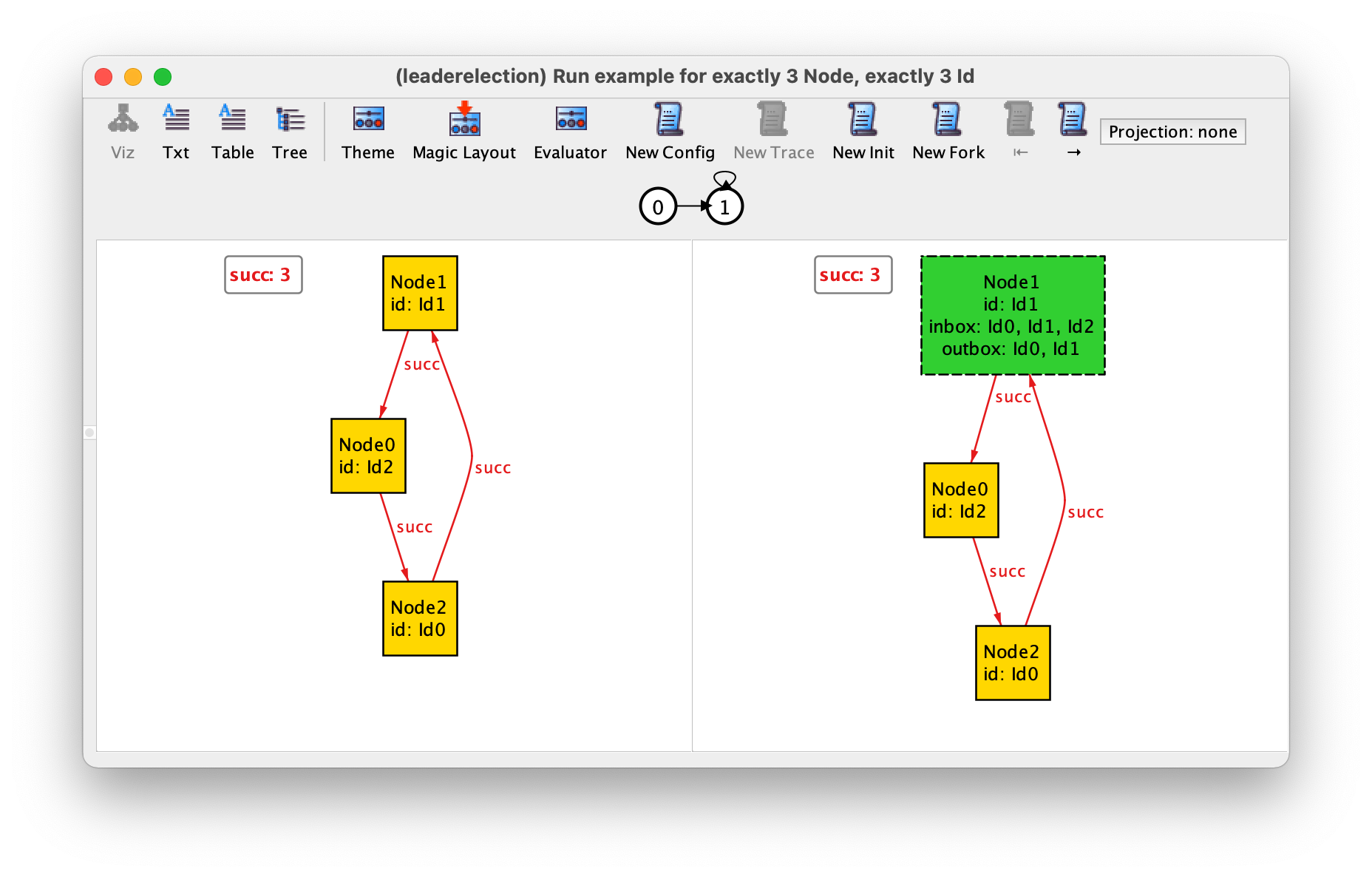
This trace displays a behaviour that should not be allowed in a correct execution of the protocol: in the second state all of a sudden several identifiers appeared in the inbox and outbox of Node1. Moreover this node was also randomly designated as leader. So far this is allowed because we added no constraints to our specification that restrict how the system can transition from one state to another. If there are no constraints then any transition is possible.
The simplest way to constraint the valid transitions is to consider all the possible events that can occur in the system, and for each event specify when it can occur (its guard) and what is its effect on the mutable relations. In our protocol we can distinguish three possible events:
a node initiates the execution by sending its own identifier to the next node.
a node reads and processes an identifier in its inbox, decides whether it should be propagated or discarded and, if it is its own identifier, elects itself as leader.
the network sends one message in the outbox of a node to the next one.
Again, Alloy has no special keywords to declare events. A common approach to do so is to declare a predicate for each event, that specifies its guard and effect, and add a constraint enforcing that at each possible state only one of those predicates can hold. Event predicates can be also parametrised, in particular by the node where the event occurs.
Let’s begin by specifying the initiate event. For each event we should
always start by specifying what is its guard, a constraint on the
current (or pre-) state that determines when can the event occur. To simplify our
specification, for the moment, we will assume that a node is free to initiate (or
reinitiate) the protocol whenever it wants, so in this case there will
be no guard, meaning the event is always possible. Then we should
specify the effect of the event on all mutable relations of the specification:
note that if nothing is said about a particular mutable relation then
its value can change freely when the event occurs. A special effect is
forcing the value of a mutable relation to not change at all,
something known as a frame condition. For example in this event we
will have two frame conditions, since it does not change the value of
inbox nor Elected. To specify that a relation does not
change with a logic formula we need to refer to its value in the next
(or post-) state. In Alloy the value of a relation (or relational
expression) in the next state is accessed by appending a prime. So, to
state that, for example, the relation inbox does not change we
could add the constraint inbox' = inbox. Likewise for
Elected. So far, the specification of event initiate looks as
follows.
pred initiate[n : Node] {
  // node n initiates the protocol

  inbox'   = inbox                           // frame condition on inbox
  Elected' = Elected                         // frame condition on Elected
}
We now need to specify the effect on relation outbox. We can
start by specifying its effect on the outbox of the initiating
node. Expression n.outbox denotes the set of identifiers in
the outbox of node n in the current state. The effect
of this event on this set is to add n’s own identifier, which
can be specified by n.outbox' = n.outbox + n.id. Here we used
the set union operator + to add the singleton set n.id
to n.outbox. Note that requiring n.id to be present in
the outbox in the next state, which could be specified by n.id
in n.outbox', is not sufficient, as it would allow identifiers other than n.id
to be freely removed or added from n.outbox. Having specified
the effect on the outbox of n we now need to specify the
effect on the outbox of all other nodes. Again, if nothing is
said about those, they will be allowed to vary freely. Of course this
event should not modify the outboxes of other nodes, something we
could specify with constraint all m : Node - n | m.outbox' =
m.outbox, that quantifies over all nodes except the initiating one. The final specification of our event looks as follows.
pred initiate[n : Node] {
// node n initiates the protocol
n.outbox' = n.outbox + n.id // effect on n.outbox
all m : Node - n | m.outbox' = m.outbox // effect on the outboxes of other nodes
inbox' = inbox // frame condition on inbox
Elected' = Elected // frame condition on Elected
}
Other, shorter or clearer ways to specify effects and frame conditions are presented in Section Specifying frame conditions. In the remainder of this chapter, we will continue to use the more verbose style, but you are highly encouraged to use a terser style once it is familiar.
To validate our first event we can impose a restriction stating that,
for the moment, this is the only event that can occur, and inspect the
possible instances to see if the system behaves as expected. To
specify such a restriction we need the temporal logic operator
always to enforce a formula to be true at all
possible states. In particular, to enforce that, at every possible
state, one of the nodes initiates the protocol, the following
fact can be added to the specification.
fact {
  // possible events
  always (some n : Node | initiate[n])
}
Running command example yields the following trace, where
Node2 initiates the protocol and then nothing else happens.
On first glance, this may seem like an invalid trace, given that we
required that at every state one node initiates the protocol. However,
if we look closely at our specification of event initiate we
can see that it also holds true in a state where a node already has
its own identifier in the outbox, which
will remain in the outbox. Our specification did not had a guard forbidding
this occurrence of the event, and the effect n.outbox' =
n.outbox + n.id is also true if n.id is already in
n.outbox and in n.outbox'.
To address this issue we could add a guard like n.id not in
n.outbox to the specification of initiate. However, this
only forbids a node from initiating the protocol if it’s own
identifier is at the moment in its outbox. This means that, once we
include an event to send messages and this identifier leaves the
outbox, a node will be able to reinitiate the protocol. This does not
pose any problem concerning the correctness of this particular
protocol, but if we really wanted each node to initiate the protocol
only once we would need to strengthen this guard.
One possibility would be to add a field to record at which phase of the protocol execution each node is in, and allow this event only when a node is in an “uninitiated” phase. This would be the common approach in most formal specification languages. However, with Alloy we have a more direct alternative. Since there is no special language to specify events and they are specified by arbitrary logic formulas, we are free to use temporal operators to specify guards or effects. By contrast, in most formal specification languages we can only specify the relation between the pre- and post-state.
In this case we could, for example, use the temporal operator
historically, that checks if something was always true in the
past up to the current state, to only allow initiate to occur
if the node’s identifier was never in its outbox. The specification of
our event would look as follows.
pred initiate[n : Node] {
// node n initiates the protocol
historically n.id not in n.outbox // guard
n.outbox' = n.outbox + n.id // effect on n.outbox
all m : Node - n | m.outbox' = m.outbox // effect on the outboxes of other nodes
inbox' = inbox // frame condition on inbox
Elected' = Elected // frame condition on Elected
}
Unfortunately, after adding this guard our command will return no trace, meaning there are no behaviours that satisfy our constraints. This happens because we are currently not allowing messages to be sent or read, so after all nodes have initiated the protocol nothing else is allowed to happen by our specification, and it is impossible to obtain a valid trace. Recall that traces are infinite sequences of states, where the system is always evolving. A simple way to solve this issue is to add an event allowing the system to stutter, that is to do nothing (keeping the value of all relations unchanged). Stuttering can also be understood as an event specifying something else that is occurring on the environment outside the scope of our specification, and in general it is a good idea to add such stuttering events. In this case, a predicate to specify a stuttering event can be specified as follows.
pred stutter {
  outbox'  = outbox
  inbox'   = inbox
  Elected' = Elected
}
To allow this event we need to change the above fact that restricts the possible behaviours.
fact {
  // possible events
  always (stutter or some n : Node | initiate[n])
}
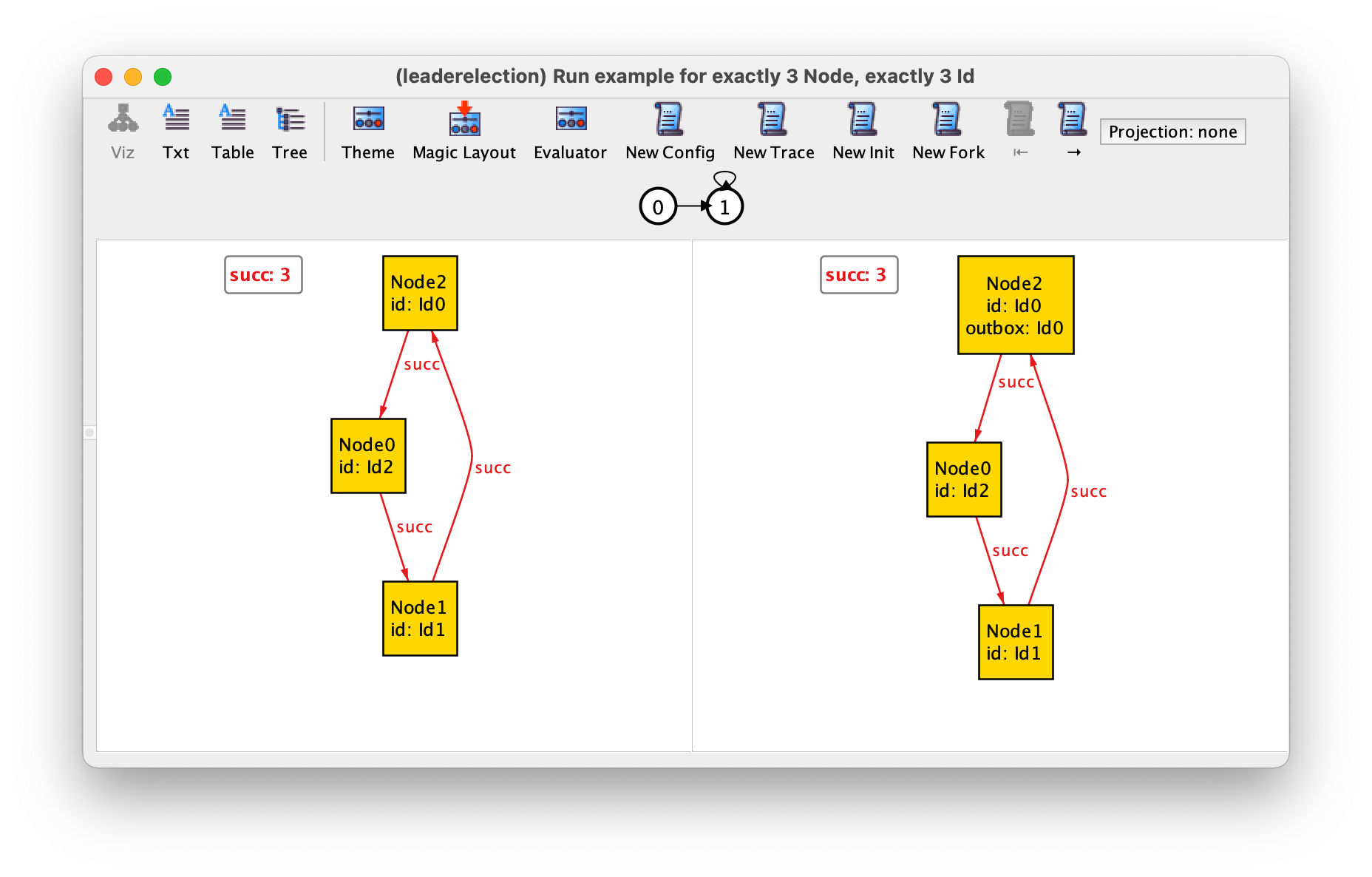
Running command example returns a trace where nothing happens
in our system, something that is now allowed. If we press
New Fork we might get a trace such as the previously
depicted, where Node2 initiates the protocol and then nothing
else happens. If we move to the next state by pressing →,
and fork again with New Fork, we might get the following
trace where Node0 initiates the protocol after Node2.
By exploring a bit more the possible traces we can get some confidence
that event initiate is well specified.
Let us now specify the send event. In this event we could have as parameters the node
n from where the message will be sent and the message
i that will be sent (an identifier). The guard of this event
should require i to be in the outbox of n. The
effect will be to remove i from the outbox of
n, and add it to the inbox of the next node n.succ. All
other inboxes and outboxes should keep their value, as well as the
Elected set. The specification of this event would be the following.
pred send[n : Node, i : Id] {
  // i is sent from node n to its successor

  i in n.outbox                              // guard

  n.outbox' = n.outbox - i                   // effect on n.outbox
  all m : Node - n | m.outbox' = m.outbox    // effect on the outboxes of other nodes

  n.succ.inbox' = n.succ.inbox + i           // effect on n.succ.inbox
  all m : Node - n.succ | m.inbox' = m.inbox // effect on the inboxes of other nodes

  Elected' = Elected                         // frame condition on Elected
}
For event process again we could have as parameters the node
n and the message i to be
read and processed. The guard should require that i is in the
inbox of n. The effect on inbox is obvious:
i should be removed from the inbox of n and
all other inboxes should keep their value. The effect on the
outbox of n depends on the whether i is
greater than n.id: if so, i should be added to the
outbox, to be later propagated along the ring; if not, it
should not be propagated, meaning the outbox of n will
keep its value. To write such conditional outcome we could use the
logical operator implies together with an else:
C implies A else B is the same as (C and A) or (not C
and B), but the former is easier to understand. The event has no
effect on the outboxes of other nodes, which should all keep their
value. The same conditional outcome applies to Elected: if the
received i is equal to the n’s own identifier, then
n should be included in Elected; else Elected
keeps its value. The full specification of process is as
follows.
pred process[n : Node, i : Id] {
  // i is read and processed by node n

  i in n.inbox                                // guard

  n.inbox' = n.inbox - i                      // effect on n.inbox
  all m : Node - n | m.inbox' = m.inbox       // effect on the inboxes of other nodes

  gt[i,n.id] implies n.outbox' = n.outbox + i // effect on n.outbox
             else    n.outbox' = n.outbox
  all m : Node - n | m.outbox' = m.outbox     // effect on the outboxes of other nodes

  i = n.id implies Elected' = Elected + n     // effect on Elected
           else Elected' = Elected
  }
We should now add these two events to the fact that constraints the valid behaviours of our system.
fact {
  // possible events
  always (
    stutter or
    some n : Node | initiate[n] or
    some n : Node, i : Id | send[n,i] or
    some n : Node, i : Id | read[n,i]
  )
}
Before proceeding to the verification of the expected properties of
the protocol, we should play around with the different instance
exploration buttons to explore different execution scenarios and
validate the specification of our events. An alternative would be to
ask for specific scenarios directly in a run command. For
example, we could change command example to ask directly for a
scenario where some node will be elected. To do so we need to use the
temporal operator eventually, which checks if a formula is
valid at some point in the future (including the present state). Our
command would look as follows.
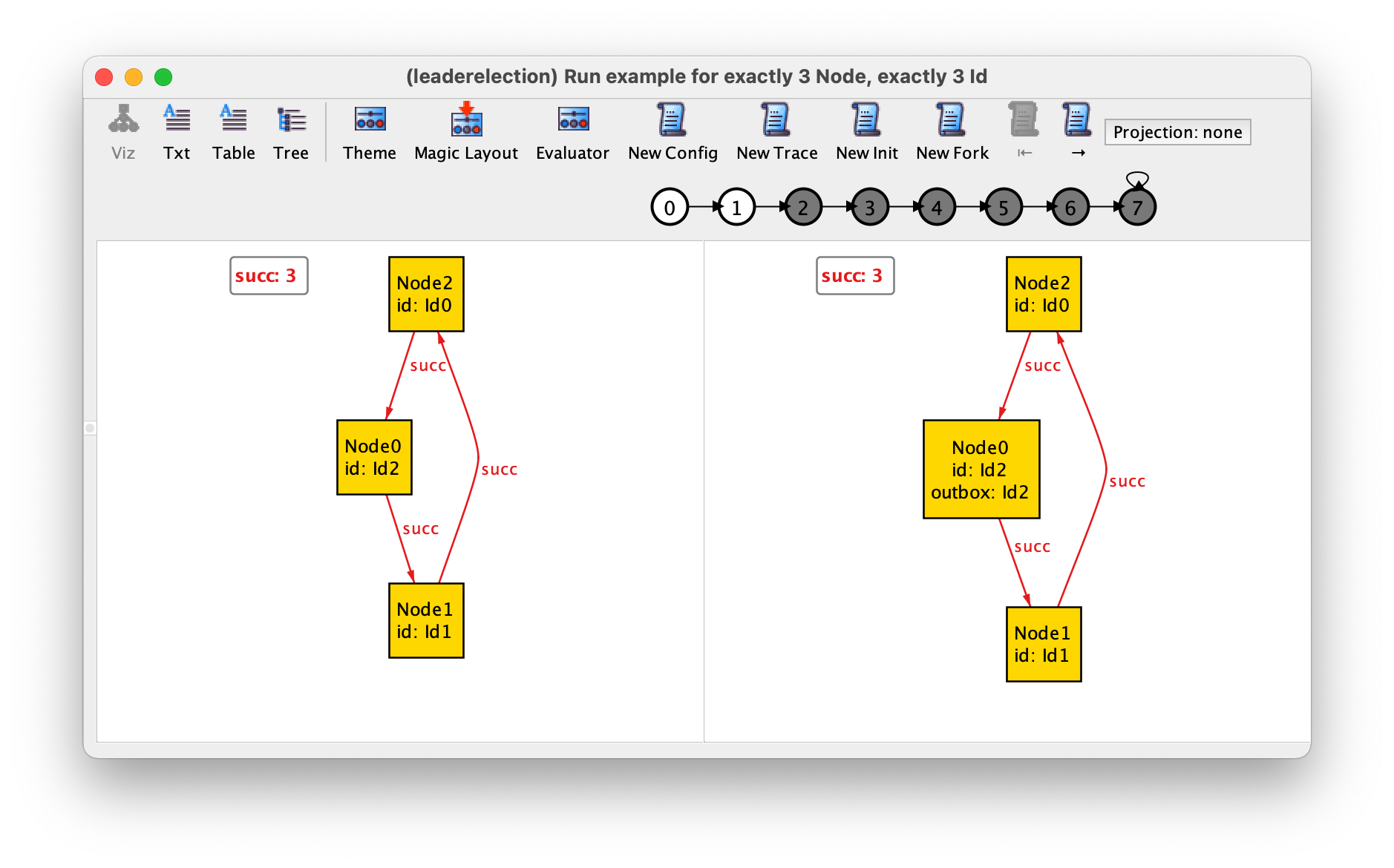
run example {
  eventually some Elected
} for exactly 3 Node, exactly 3 Id
Running this command will return a trace with 8 states where the highest identifier is passed around until the respective node gets elected. This is the shortest trace where a leader can be elected in a ring with 3 nodes, corresponding to one initiate event followed by 3 interleaved send and read events. The Analyzer guarantees that the shortest traces that satisfy (or refute) a property are returned first. The first transition of this trace is the following, where the node with the highest identifier initiates the protocol.
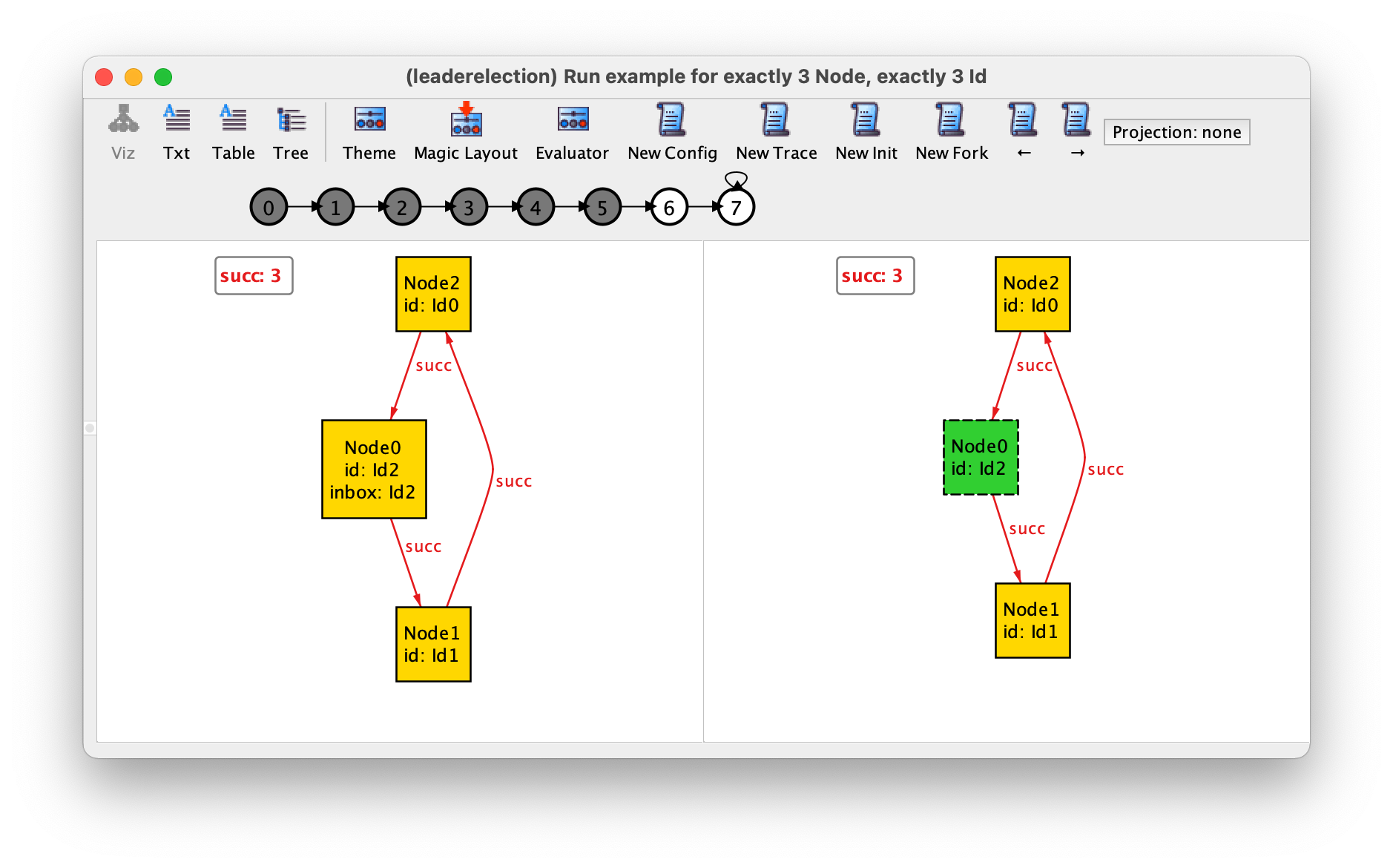
In the last transition, that can be focused by pressing → 6 times or by directly clicking the state numbered 6 in the trace depiction, the node with the highest identifier reads its own identifier that was passed around in the ring and elects himself as leader.
Verifying the expected properties of the protocol
The key property of our protocol is that eventually exactly one node will become leader. We can break this property into to simpler ones:
There will never be more than one leader
Eventually there will be at least one leader
These properties are of very different nature: the former is a safety property, forbidding some (undesired) behaviour of the system, while the latter is a liveness property, forcing some (desirable) behaviour of the system. The analysis of safety properties is usually simpler than the analysis of liveness properties. To find a counter-example for a safety property it suffices to search for a finite sequence of states that leads to a (bad) state (in this case one where there are two or more leaders), and it is irrelevant what happens afterwards, as any continuation of this finite sequence will still be a counter-example. On the other hand, to find a counter-example for a liveness property it is necessary to search for a complete infinite trace where the expected behaviour definitely never happened (in this case a leader is never elected). Moreover, it will be necessary to impose additional fairness conditions when verifying liveness properties, in particular to forbid bogus counter-examples where at some point the system stutters forever and thus the expected behaviour never happens.
Let us start by verifying the first (safety) property. Recall that
properties that are expected to hold should be written in named
assertions (declared with keyword assert) and then verified
with check commands. This safety property is a very simple
example of an invariant, a property that requires something to be
be true in all states of all possible traces. In Alloy, invariants can
be specified using the temporal operator always. In each state, to check that
there is at most one leader in set Elected we could use
the keyword lone. This invariant could thus
be specified as follows.
assert AtMostOneLeader {
  always (lone Elected)
}
To check this assertion we could define the following command.
check AtMostOneLeader
This protocol is known to be correct, so, as expected, running this command returns no counter-example. Recall that the default scope on top-level signatures is 3, so this command verifies in a single execution that the property holds for all rings with up to three nodes. Moreover, by default, verification of temporal properties is done with a technique known as bounded model checking, meaning that the search for counter-examples will only consider a given maximum number of different transitions before the system starts exhibiting a repeated behaviour. By default this maximum number is 10. To increase our confidence in the result of the analysis we could, for example, check this property for all rings with up to 4 nodes and consider up to 20 different transitions (or steps). To do so we could change the scope of the command as follows.
check AtMostOneLeader 4 but 20 steps
This commands sets the default scope on signatures to 4 but also
changes the scope on transitions to 20 using keyword
steps. Again, as expected, no counter-example is returned, but
the analysis now takes considerably longer, as there are many more
network configurations and states to explore.
It is also possible to check a temporal property with unbounded model
checking, taking into consideration an arbitrary number of
transitions, but still with the signatures bounded by a maximum
scope. To do so, a special scope on steps is needed
to trigger unbounded temporal analysis.
check AtMostOneLeader 4 but 1.. steps
However, for such analysis to be performed it is necessary to select a solver in the
menu that supports it. By default, the Alloy Analyzer is not pre-packaged with
solvers that support unbounded model checking. You first need to
install either the NuSMV or the nuXmv model checker, and then select
Electrod/NuSMV or Electrod/nuXmv as solver,
respectively. The Analyzer shows that the safety property holds even
with an arbitrary number of transitions.
The second property is also a very simple example of a liveness
requirement, namely one that requires something to hold at least in
one state of every trace. Such properties can be specified directly
with the temporal operator eventually. Inside this temporal
operator, again a very simple cardinality check on Elected
suffices, this time with keyword some.
assert AtLeastOneLeader {
  eventually (some Elected)
}
The following command can be used to check this property with bounded model checking and the default scopes.
check AtLeastOneLeader
Both Electrod/NuSMV and Electrod/nuXmv can be used to check this command, since they also support
bounded model checking. Alternatively, we can also choose one of the SAT solvers
pre-packaged with the Analyzer in the menu, for example the SAT4J
solver. Feel free to experiment with different solvers when analysing
a property, as the performance can sometimes vary significantly just
by choosing a different solver. We recommend that you start by
verifying specifications with bounded model checking, because it is
usually much faster than the unbounded counterpart, and most
counter-examples tend to require only a handful of transitions. Once
you have a design where no counter-example is returned with bounded
model checking, you can increase your confidence on the analysis by using
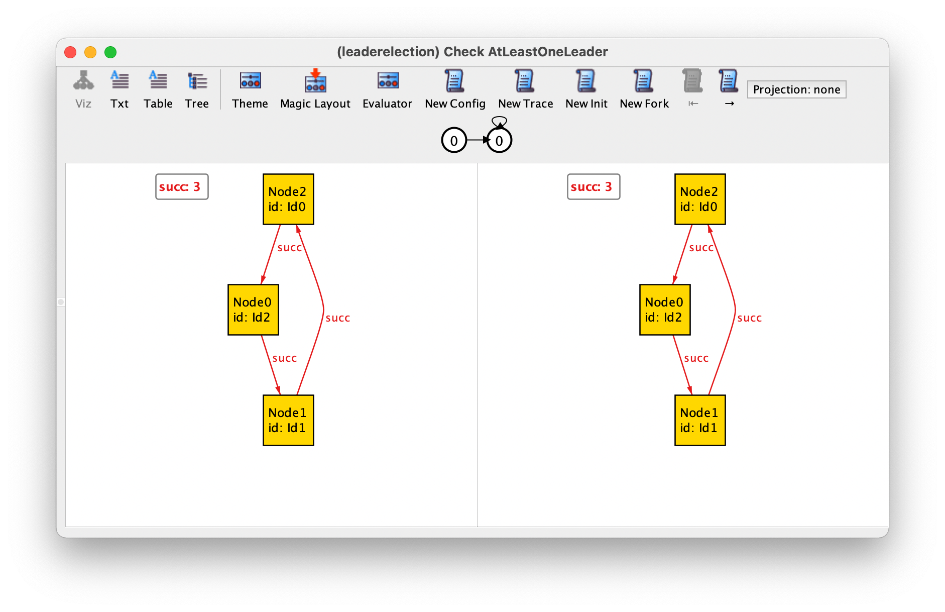
unbounded model checking. As hinted above, running this command immediately returns a
counter-example where the system stutters forever, and obviously no
leader is elected.
This behaviour is allowed because we added a stutter event that captures events external to our system. At the moment this event can occur indefinitely, which is a bit unrealistic or unfair to the system under analysis: for example, if at some point the system is continuously ready to execute an event (the event is continuously enabled), then it should eventually occur. For example, in our protocol, a trace where at some point a message is in the inbox of a node but is never read is unfair to that node.
To specify such fairness properties we first need to understand two
well-known combinations of the always and eventually
temporal operators:
eventually always pholds in a system if all traces reach a state wherepbecomes valid indefinitely.always eventually pholds in a system if in every state of every tracepis later valid, which means thatpis true infinitely often.
To specify that an event is at some point continuously enabled we can
use the first combination. But first we need to specify when is a
particular event enabled (ready to occur). Most of the times this
condition is exactly the same as the guard of the event, but in some
events there can be additional conditions that derive from its
effect. In our protocol, the enabled condition for all events is the
same as the guard. For example, given a node n and identifier
i, event process[n,i] is enabled when i in
n.inbox. So, to specify that event
process[n,i] becomes continuously enabled at some point we
could write eventually always i in n.inbox. However, if, for example, the outbox of a node was limited
to contain at most one identifier, then we would have additional
enabling conditions, as the effect n.outbox' = n.outbox + i
that occurs when gt[i,n.id] would also require that
n.outbox is empty.
To specify that a continuously enabled event eventually occurs (after
the point it becomes enabled) the second combination of
operators presented above can be used. Note that a continuously enabled event
would still be (continuously) enabled after the required occurrence of
the event, which means that the event should occur again and again, or
infinitely often. So, the desired fairness condition for
event process[n,i] can be specified as follows.
(eventually always i in n.inbox) implies (always eventually process[n,i])
Technically, this fairness condition is known as weak fairness, as
the event is only required to happen if continuously enabled. Often
this suffices to verify most liveness properties. However, sometimes
we may need strong fairness constraints, requiring that the event
occurs when it becomes recurrently enabled (infinitely often, but
not necessarily continuously). For event process[n,i] such strong fairness
constraint would be specified as follows.
(always eventually i in n.inbox) implies (always eventually process[n,i])
In our example property, the liveness property holds if we require weak fairness for all instances of three events of the system, as specified in the following predicate.
pred fairness {
all n : Node, i : Id {
(eventually always historically n.id not in n.outbox) implies (always eventually initiate[n])
(eventually always i in n.inbox) implies (always eventually process[n,i])
(eventually always i in n.outbox) implies (always eventually send[n,i])
}
}
Finally, if we change the AtLeastOneLeader assertion to assume
fairness, no counter-example will be returned even with increased
scopes, as expected.
assert AtLeastOneLeader {
fairness implies eventually (some Elected)
}
To better understand fairness constraints, suppose we commented
out the fairness restriction on event process.
pred fairness {
all n : Node, i : Id {
(eventually always historically n.id not in n.outbox) implies (always eventually initiate[n])
-- (eventually always i in n.inbox) implies (always eventually process[n,i])
(eventually always i in n.outbox) implies (always eventually send[n,i])
}
}
The check AtLeastOneLeader command would immediately return a
counter-example in a configuration with a single node, that initiates
the protocol, sends its own identifier to himself, and then never
processes that identifier (something that would be allowed at this point, since neither initiate nor read are enabled).
The last two states before the trace starts stuttering are shown below.
This trace is fair to initiate and send, but not to
read, which is always enabled in the stuttering part of the
trace but never occurs.
Warning
Avoid fairness conditions in facts!
Instead of a predicate we could have specified the fairness
conditions inside a fact, to force them to be true in all
analyses. However, in general that is not a good idea, since
run commands would then only return fair traces, which
hinders the interactive exploration of scenarios and requires
much larger bounds on the number of steps (making the analysis
slower). For example, command
run {} for exactly 3 Node, exactly 3 Id
that asks for any trace in a ring with 3 nodes will not even return
a trace with the default scope of 10 steps, because no fair
trace with this size exists for this configuration. The minimum
scope would be 14 steps!
This also means that a command like check AtMostOneLeader,
to verify the safety property of the protocol, would be mostly
pointless, as with the default scope of 10 steps only
configurations with up to 2 nodes would be checked for
correctness. Without fairness imposed in a fact, it would at least
check that the safety property is not violated in the first 10
steps of any trace of the protocol, including unfair and fair
ones. Recall that in a counter-example of a safety property it is
irrelevant what happens after we reach a faulty state: any
continuation of the “bad” trace prefix would still be a
counter-example, including any fair continuation.
Making the specification more abstract
Caution
This section is still under construction
open util/ordering[Node]
sig Node {
succ : one Node,
var inbox : set Node
}
fact {
// at least one node
some Node
}
fact {
// succ forms a ring
all n : Node | Node in n.^succ
}
fact {
// initially inbox is empty
no inbox
}
fun Elected : set Node {
{ n : Node | n not in n.inbox and once (n in n.inbox) }
}
pred initiate[n : Node] {
// node n initiates the protocol
historically n not in n.succ.inbox // guard
n.succ.inbox' = n.succ.inbox + n // effect on n.succ.inbox
all m : Node - n.succ | m.inbox' = m.inbox // effect on the inboxes of other nodes
}
pred process[n : Node, i : Node] {
// i is read and processed by node n
i in n.inbox // guard
n.inbox' = n.inbox - i // effect on n.inbox
gt[i,n] implies n.succ.inbox' = n.succ.inbox + i // effect on n.succ.inbox
else n.succ.inbox' = n.succ.inbox
all m : Node - n.succ - n | m.inbox' = m.inbox // effect on the inboxes of other nodes
}
pred stutter {
inbox' = inbox
}
fact {
// possible events
always (
stutter or
some n : Node | initiate[n] or
some n : Node, i : Node | process[n,i]
)
}
run example {
eventually some Elected
} for 3 Node
assert AtMostOneLeader {
always (lone Elected)
}
check AtMostOneLeader for 5 but 1.. steps
pred fairness {
all n : Node, i : Node {
(eventually always historically n not in n.succ.inbox) implies (always eventually initiate[n])
(eventually always i in n.inbox) implies (always eventually process[n,i])
}
}
assert AtLeastOneLeader {
  fairness implies eventually (some Elected)
}
check AtLeastOneLeader for 3 but 1.. steps
Exercises
To practice temporal logic, access the following Alloy4Fun model and specify all the listed constraints. Each constraint is specified in a separate predicate, and for each there is a command that can be used to check its correctness. If the constraint is not correctly specified a counter-example will be shown. The counter-example will include an atom that clarifies if it is an example that the incorrect constraint is currently rejecting but should be accepted or one that is currently being accepted but should be rejected. Unlike in the Alloy Analyzer, in Alloy4Fun only one state of the trace is shown at a time. Use the green arrows to navigate back and forward in the trace. In the last state of the trace before looping back the forward arrow is circle shaped.
Specify Dijkstra’s self-stabilizing mutex algorithm, that works on arbitrary rings of
N+1machines, with a distinguished bottom machine. In particular, specify the solution withKstate machines, both with and without a central daemon. The central daemon ensures that only one machine with the privilege executes at each time, otherwise an arbitrary number of machines can execute. The rules for determining if a machine has the privilege to execute are as follows: the bottom machine has the privilege if its state is equal to that of its neighbor; a non-bottom machine has the privilege if its state is different from that of its neighbor. When the bottom machine executes it increments its state moduloK. When a non-bottom machine executes it just copies the state of its neighbor. The goal is to verify the expected convergence and closure properties. Convergence is a liveness property that ensures that whatever the initial state, the system will converge to a legitimate global state. In this case, a legitimate global state is one where exactly one machine has the privilege to execute and where every machine will eventually obtain that privilege. Closure is a safety property that ensures that after reaching a legitimate global state, the system will forever stay in a legitimate global state. According to the paper, without a central daemon both convergence and closure hold whenK > N, while with a central daemon it suffices thatK >= N. Use the Alloy Analyzer to verify if that is indeed the case. Notice that instead of using integers to model the local states of the machine, a ring ofKvalues can be used.Specify Chang’s echo distributed protocol for forming a spanning tree in an arbitrary connected network with a distinguished initiator. In particular, specify Algorithm 0 described in the paper, that works roughly as follows. The initiator starts by sending an explorer message to all its neighbors. Upon receiving a message, each node acts as follows:
If the message is an explorer and it is the first to arrive at the node, mark the sender as the first neighbor and send an explorer to all neighbors except the first. Note that it is assumed that the initiator is considered to have been explored a priori.
If the message is an explorer but is not the first to arrive or there are no neighbors except the first, send an echo message back to the sender.
If the message is an echo, register that an echo as been received from the sender, and if echos from all neighbors (to which explorers were sent) have arrived send an echo to the first neighbor, unless the node is the initiator, in which case the protocol is finished.
Verify the expected properties of the protocol, namely that it will eventually finish and that when it finishes the first relationship defines a spanning tree of the network rooted at the initiator.